An agent designed a maritime search radar and beat my reference on cost
Yesterday I gave a coding agent a radar design brief and a scoring harness that does not care what the agent says about itself. The task: architect an X-band phased-array search radar that detects small boats in sea clutter, sweeps its assigned volume inside a three second frame budget, stays under power and cost ceilings, and still meets its availability floor after months of component failures. Nine requirements, scored from physics over test conditions the agent never sees.
The first attempt passed all nine, in 28 turns and about eight minutes, at an API-equivalent cost of $1.03, and the design it submitted was cheaper than the reference solution I had built for the task. Five more attempts followed, and four of the six passed. For the first time in this project I can also show how they worked, because the harness now records every tool call the agent makes and every physics call its code triggers, in every process, including the model servers.
This is the third post in a series. The first was about an agent finding a flaw in my benchmark. The second laid out the open-source stack. This one is about the stack doing the thing it was built for.
Why search radar is a good test
A search radar architecture is a knot of couplings, which is what makes it a better test than any single-discipline problem.
Make the aperture bigger and the beam gets narrower, which helps detection twice: more gain, and a smaller clutter cell. But a narrower beam needs more beam positions to tile the search volume, and each position costs a dwell, so the frame time grows until the radar can no longer revisit its volume inside the budget. Integrate more pulses per dwell and you buy detection sensitivity, but the dwell gets longer and the frame problem gets worse. Cut pulses and you must recover the sensitivity with per-element power, which heats the transmit/receive modules; the reliability model derates component life with junction temperature, so a hot design fails its availability floor months into the mission. The power amplifier class couples three ways at once: a cheap PA is inefficient, runs hot, and has the shortest rated life.
The waveform is part of the submission, but the duty cycle is not: it is computed from the submitted pulse repetition frequency and a pulse width the task pins. Submitting a duty cycle is an error. In the first post I called axes like this the free lunch: any quantity that helps the score, costs nothing in the model, and would be an engineering decision in real life has to be priced or pinned, or an optimizer, human or agent, will quietly max it out.
The rules
The task ships as a brief plus a deliverable contract: one YAML file naming the array geometry, taper, phase resolution, PA class, per-element power, PRF, pulses per dwell, and the digitization scheme. The evaluator recomputes every metric from that file. Detection probability is scored worst-case over an envelope of test points, target range and size, scan angle, sea state, plus five seeded random element-failure draws, and the brief declares only the bounds of that envelope, never the points or the seeds.
Two independent checks run on every evaluation. Antenna gain and sidelobes are recomputed by full pattern integration with a separate antenna library, with the quantization and failure draws applied. And the detection probability at the binding test point is recomputed by Monte Carlo: two hundred thousand draws of a fluctuating Swerling-1 target through an actual cell-averaging CFAR detector, with the threshold set from exact false-alarm statistics. The Monte Carlo shares no code with the analytic detection chain it checks.
What calibration turned up before any agent ran
Freezing the task’s thresholds from measurement surfaced two things worth recording.
First, the analytic chain models CFAR as a fixed SNR loss, calibrated for single-pulse detection. The Monte Carlo showed that approximation is conservative when pulses are integrated, by up to 0.09 in detection probability in the operating region, because the CFAR’s noise estimate gets better as its reference cells integrate more pulses and the fixed loss does not shrink to match. The disagreement is one-sided in the safe direction, and the cross-check tolerance is frozen just above the measured worst case.
Second, the scenario I originally wrote was impossible. I wanted the radar hunting low-flying aircraft over sea clutter at 40 to 60 km. The models said no design in the entire space could do it, and they were right to say so: the task’s detection chain integrates pulses noncoherently and has no Doppler processing, and without Doppler there is no way to separate a slow, low target from kilometers-wide clutter cells. Real radars solve this with MTI and pulse-Doppler filtering, which my system models do not yet represent. So the scenario became what the model space can honestly support: small surface craft inside the radar horizon, where geometry keeps the clutter workable. A benchmark task has to live inside its models’ validity, and finding the edge of that validity is most of the work of writing one.
The runs
I ran six attempts in two arms: three with the physics libraries importable and nothing else, three with the phased-array-systems and APAB MCP servers attached. Same model, same task, same thirty-minute limit.
| arm | outcome | design | est. cost | wall |
|---|---|---|---|---|
| MCP | pass | 64 × 32, class B, 6.0 W, 32 pulses | $1.03 | 468 s |
| MCP | pass | 40 × 40, class C, 7.0 W, 64 pulses | $2.14 | 1172 s |
| MCP | pass | 64 × 32, class B, 8.0 W, 32 pulses | $2.46 | 648 s |
| library | fail (frame time) | 48 × 48, class B, 9.0 W, 36 pulses | $4.89 | 1295 s |
| library | pass | 48 × 48, class B, 4.0 W, 56 pulses | $4.66 | 1612 s |
| library | timeout | no submission | $4.43 | 1800 s |
Three of three with tools attached, one of three without, at roughly a third of the cost and half the wall time. That is the same direction I measured on the satellite terminal task two days earlier, so it is now two tasks pointing the same way.
Then I looked at the transcripts, and the obvious explanation fell apart. The MCP-attached agents made 1, 0, and 1 MCP tool calls across the three attempts. Whatever separates the arms, it is not that one group used the tools and the other did not. Almost nobody used the tools.
What does separate them is visible in the physics call log: 238, 1714 and 1009 instrumented model calls in the MCP arm against 3062, 8187 and 30,602 in the library arm. The attempt that timed out was still sweeping parameters at thirty minutes with thirty thousand pattern computations behind it. The library agents spent their budget building and running their own search loops. The tool-attached ones converged sooner.
I have a hypothesis I cannot test with three attempts per arm. When the servers are attached, their tool schemas sit in the agent’s context: parameter names for Swerling case, CFAR type, clutter model, search extents, PRF. That is a menu of the variables the system model actually prices, readable without calling anything. An agent that sees the menu may stop guessing at what matters sooner. It is equally possible that six runs of a stochastic process gave me a pattern that will not survive twenty. I am reporting the numbers with that caveat attached rather than choosing the flattering reading.
Aperture shape split the arms cleanly. Both 64 × 32 designs came from the MCP arm, and they are the two cheapest passing designs on record for this task, $482,560 and $486,400 against my reference’s $512,928. Both library attempts that submitted anything chose a square.
The cheapest attempt is worth walking through. The agent read the brief, called the system model’s MCP evaluation tool once to check a candidate against the nominal scenario, then wrote its own scripts to sweep the geometry, 234 logged pattern computations, and submitted this:
- 64 × 32 aperture, half-wavelength spacing
- Taylor taper at −30 dB, 5-bit phase shifters
- class B power amplifiers at 6.0 W per element
- PRF 2000 Hz, 32 pulses per dwell
My reference is a 48 × 48 square at 6.3 W with the same PA class and waveform. Both pass everything. The agent’s design costs $486k against the reference’s $513k and draws 3,859 W against 4,523 W.
The interesting part is the shape. Sea clutter competes with the target inside one resolution cell, and the cell’s azimuth width is range times beamwidth. Stretching the aperture in azimuth narrows exactly the beamwidth that sets the clutter cell, while the elevation dimension, which contributes gain but not azimuth resolution, stays small and cheap. Fewer elements, arranged where they matter.
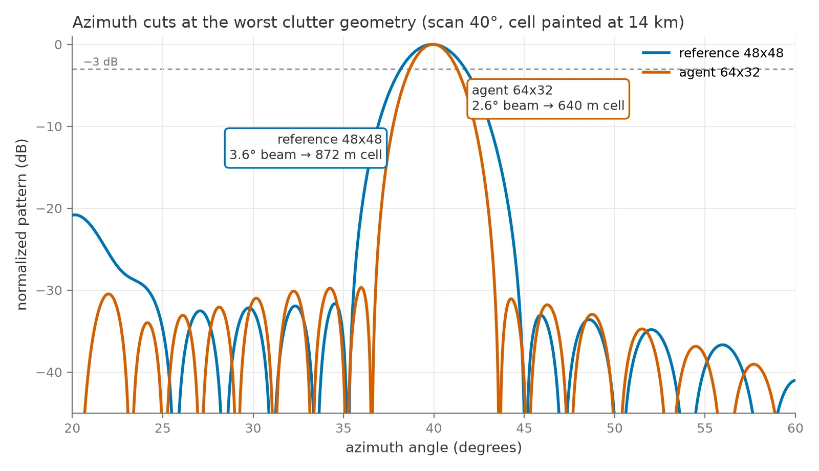
Both patterns recomputed with the independent antenna library at the task’s worst clutter geometry. The agent’s 64 × 32 aperture cuts the azimuth beamwidth from 3.6° to 2.6°, shrinking the clutter cell it paints at 14 km from 872 m to 640 m, about 1.3 dB of signal-to-clutter ratio that costs no transmit power. The figure script recomputes these numbers before drawing them.
One wrinkle belongs in the record: my reference solver never considered this shape, because I wrote its search grid over square apertures only. The agent did not outsmart physics I understood; it searched an axis I had left out. I find that more encouraging than a win against a stronger reference would have been, because the failure it exposes, a human quietly narrowing the design space out of habit, is the exact failure this workflow exists to catch.
Showing the work
Earlier posts in this series had to hedge about what the agents actually did, because the harness kept no tool-call log. That gap is closed, and the run bundle for each attempt now carries three artifacts worth naming.
The transcript records every tool call with its inputs. From it the manifest derives an integrity flag, which trips if any filesystem-capable call references the task’s reference-solution directory. This run’s flag is clean, and that claim is checkable rather than taken on faith.
The physics call log records every entry into an instrumented model function, per process. For this run: four system-model evaluations at the reduced-order tier and 234 pattern computations at the aperture tier, across four separate processes, because the instrumentation now reaches inside the MCP server processes too. Whether an agent uses the provided tools or writes its own physics is now a measured property of a run. This agent did both: one MCP call to orient, then its own sweep scripts for the search.
The server-side trace records the MCP servers’ own spans, so a tool call seen by the agent can be matched to the computation the server actually ran.
What this does not show
Three attempts per arm is enough to see a direction, and nothing here is a pass rate with error bars. The schema-as-menu explanation for the gap between arms is a hypothesis I have no power to test at this sample size, and the honest alternative is that six runs of a stochastic process produced a pattern that twenty would erase. One model family ran the task. The models are closed-form system models: no Doppler processing, no waveform simulation, no measured data anywhere in the loop, and the sea clutter level comes from a published empirical model that I checked against literature ranges rather than recomputing independently. Passing the task means finding a compliant architecture under the stated couplings, and says nothing about optimality; the agent’s design is cheaper than my reference, and something cheaper than both almost certainly exists.
What this looks like in my own projects
The task, evaluator, Monte Carlo cross-check, calibration script, and every
run bundle quoted above are committed in
AEDL, with
the task definition at
tasks/t3-002-xband-search-radar.
The system models are
phased-array-systems, the pattern
cross-check is
phased-array-modeling, and the MCP
servers come from APAB and
opensatcom. The calibration story behind the task
follows the method from
the free-lunch post, and the
stack’s design rules are in
the stack post.
Try it
git clone https://github.com/jman4162/aedl-electromagnetic-design-agent aedl
cd aedl
python -m venv .venv && source .venv/bin/activate
pip install -e ".[systems]"

# score the committed reference design
python -c "
from pathlib import Path
from aedl import get_evaluator
from aedl.spec import find_task
spec = find_task(Path('tasks'), 't3-002')
result = get_evaluator(spec.evaluator)(spec, Path('tasks/t3-002-xband-search-radar/reference/architecture.yaml'))
print('pass' if result.passed else 'fail')
"

# run an agent against it (Claude Code CLI required)
aedl run --task t3-002 --agent claude --model sonnet --attempts 1
Every number above comes from committed run bundles and calibration output, re-read from disk while writing, and the figure script recomputes both patterns before drawing them. The task models are closed-form and validated against public oracles, not against measurement.
AEDL and the phased-array tools are independent projects I build on my own time. The views are my own and do not represent any current or former employer.
Frequently asked questions
What did the agent actually design?
The architecture of an X-band phased-array search radar: aperture size and shape, amplitude taper, phase shifter resolution, power amplifier class, per-element transmit power, pulse repetition frequency, and pulses per dwell. It submitted one YAML file. A deterministic evaluator recomputed every scored metric from that file alone, over test conditions the agent never saw.
How do you know the agent did not cheat or just claim success?
Nothing the agent writes in prose is scored, and the run bundle records the full tool-call transcript, an integrity flag that trips if any filesystem call touches the reference solution, and a per-process log of every instrumented physics call, including calls made inside the MCP server processes. The bundle for this run shows one MCP system-evaluation call, 234 pattern computations from scripts the agent wrote itself, and a clean integrity flag.
What does the 64 by 32 aperture buy over a square array?
Sea clutter competes with the target inside one radar resolution cell, and the cell's width is range times azimuth beamwidth. Making the array wider in azimuth narrows that beamwidth, which shrinks the clutter cell and raises signal-to-clutter ratio directly. At the task's worst clutter geometry the agent's beam paints a 640 m cell where my reference paints 872 m, worth about 1.3 dB before spending a watt.
Did the agent really beat your reference design?
Two of six attempts produced a 64 by 32 aperture that passes the same nine requirements at lower unit cost than my reference, so the result is real but it is a statement about my search space as much as about the agent. My reference solver enumerated square apertures only, so the rectangular option was never on its menu. Stated precisely, the agent beat my search space, and the interesting part is that it searched along an axis I had not thought to include.
The tool-attached agents barely called the tools. So what did the tools do?
I do not know, and the transcripts are what forced me to say so. The three attempts with MCP servers attached made one, zero and one tool calls, yet passed three for three at roughly a third the cost of the unattached arm. The difference shows up as physics calls: the unattached agents ran ten to thirty times more model evaluations building their own parameter sweeps. One hypothesis is that the tool schemas list the variables the system model prices, which is useful even unread. Three attempts per arm cannot separate that from ordinary variance.
Does this mean agents can do radar engineering?
It means one model family passed one calibrated architecture task four times in six attempts at the fidelity of closed-form system models, and the evidence for that is logged rather than narrated. The task has no Doppler processing, no signal simulation, and no measured data behind it. Detection statistics are cross-checked by Monte Carlo, but the sea clutter level comes from a published empirical model I checked against literature ranges, not from measurement.
More in AI agents
- MCP transport is a lifecycle decision · 2026-08-27
- A SysML v2 model that runs its own verification · 2026-08-21
- Data provenance for agentic AI workflows · 2026-08-17