Physics, learning, and control, in one helicopter simulator
In the late 2000s a Stanford team led by Pieter Abbeel, Adam Coates, and Andrew Ng got an autonomous helicopter to fly airshow aerobatics: flips, rolls, loops, tic-tocs, even a tail-slide and an auto-rotation landing. The interesting part was how. They did not hand-code the maneuvers or copy a single expert flight. They collected several imperfect human demonstrations of each maneuver, inferred the intended trajectory hiding inside them, identified the helicopter’s dynamics from flight data, and tracked the result with optimal control. On several maneuvers the autonomous helicopter flew the intended path more cleanly than any of the demonstrations it learned from (Abbeel, Coates & Ng, IJRR 2010).
I rebuilt the three ideas behind that result as a simulator that runs in your browser: helicopter-ml-simulator (live demo). You can fly it by hand, hand it to an autopilot, and watch each piece work. This post walks through the three pillars, physics, learning, and control, and how they fit together. (There is a shorter project page too.)
The physics
Underneath everything is a rigid-body flight model, the paper’s Eq. 1. The state is the helicopter’s position, orientation, and body-frame linear and angular velocities, and there are four controls: two cyclic inputs that tilt the rotor disk (roll and pitch), the tail rotor (yaw), and the collective (thrust). The body-frame accelerations combine gravity, the usual rigid-body coupling terms, damping, and control effectiveness, integrated with RK4 over a unit quaternion so the attitude never drifts off the sphere. The result is a helicopter you can fly with a keyboard or a gamepad.
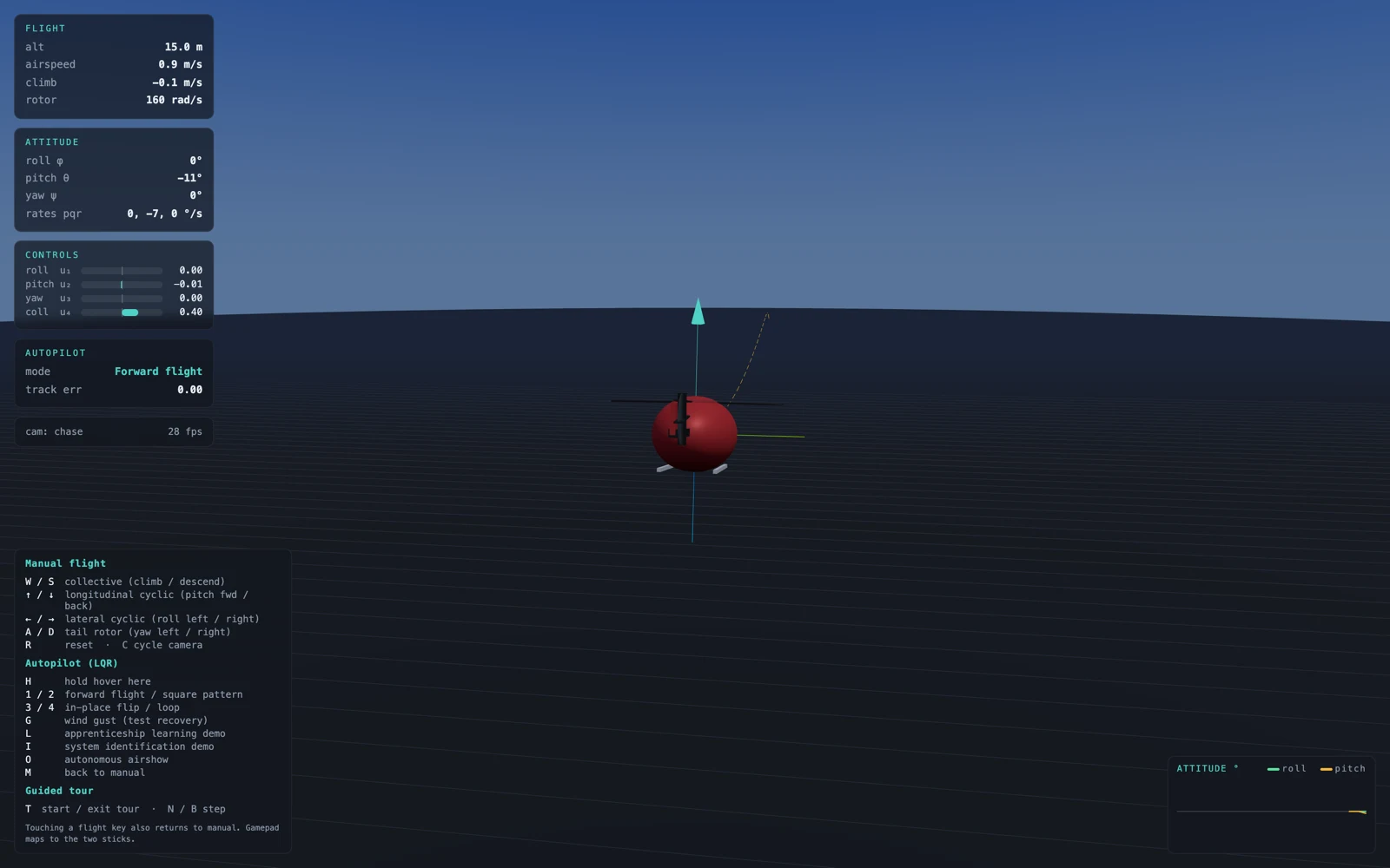
The live simulator: rigid-body flight dynamics with a stylized 3D view, live telemetry, and an autopilot. Fly it by hand or let it fly itself.
Learning the maneuver from imperfect demonstrations
This is the centerpiece. Say you want the helicopter to fly a figure-eight. You have several human demonstrations, and every one is flawed: the timing drifts, the loops come out lopsided, and no two line up. Averaging them directly does not help, because they are out of phase with each other.
Apprenticeship trajectory learning treats the maneuver you meant to fly as a hidden trajectory and recovers it with expectation-maximization. Each round does two things: it time-aligns every demonstration to the current estimate using dynamic time warping, then it fuses the aligned demonstrations with a Kalman smoother into one clean path. Alternating those two steps is the EM loop, and it converges on the intended trajectory. A useful detail from the paper: the dynamics model used for this smoothing does not have to be accurate, because the shape of the maneuver comes from the demonstrations rather than the smoothing model.
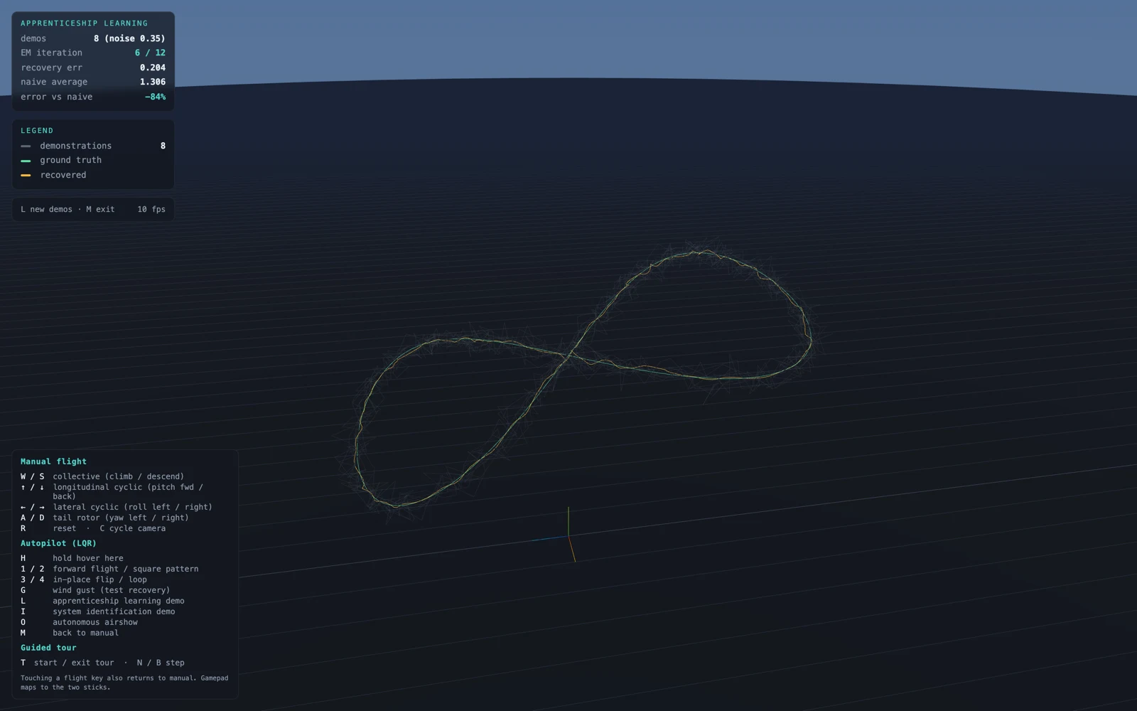
Eight noisy, time-warped demonstrations collapse to a recovered figure-eight. Because the demos are generated from a known ground-truth path, the recovery error is measurable: here about 92% below a naive average, and still dropping over the EM iterations.
In the simulator the demonstrations are synthetic, generated from a known ground-truth path with added noise and time-warping, which is what makes the recovery error measurable rather than a matter of eyeballing the curve.
Learning the dynamics from data
The control step needs a model of how the helicopter responds, and you can learn that from flight data too. The coefficients in Eq. 1, the damping terms, the control effectiveness, and the biases, all enter the accelerations linearly. So you fly a richly varied trajectory, log the states and controls, move the known kinematic terms (gravity, Coriolis, gyroscopic coupling) to one side, and regress the leftover acceleration onto the states and controls. Linear least squares recovers the coefficients.
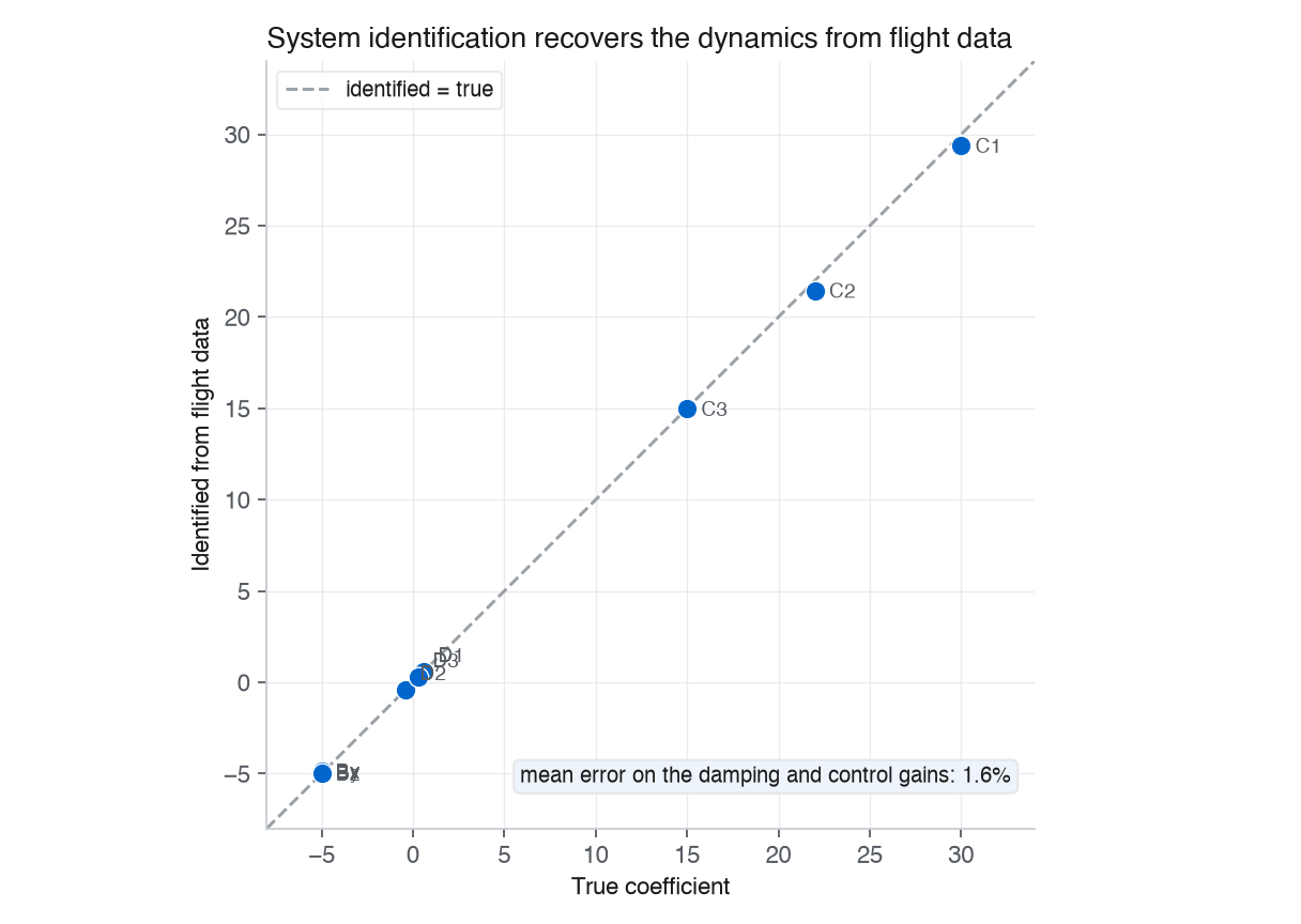
The damping and control coefficients recovered from a noisy flight log, plotted against their true values. Least squares lands within a couple of percent. From a faithful reimplementation of the identification on synthetic data.
This closes a satisfying loop: the same model the simulator integrates can be re-learned from the data it generates, to within a couple of percent.
Control that ties it together
With an intended trajectory and a dynamics model in hand, control is the classical part. A hover is held by an infinite-horizon LQR, the linear-quadratic regulator that trades off state error against control effort. Maneuvers are tracked by a time-varying LQR that linearizes the dynamics along the reference path and computes a schedule of feedback gains, which is the tracking form of the paper’s Gauss-Newton LQR. Inject a wind gust and you can watch the controller pull the helicopter back to its setpoint.
Where physics and machine learning meet
The reason this example is worth rebuilding is how cleanly the pieces interlock. Physics supplies the model. Machine learning shows up twice: once to learn the behavior (the intended trajectory, from imperfect demonstrations) and once to learn the model itself (the dynamics, from flight data). Control uses both to fly the maneuver. Each pillar is modest on its own, and together they let a helicopter fly aerobatics that no one hand-programmed. Physical models and learning working together on a real system is the thread I keep coming back to.
Fly it
The simulator is a live demo in your browser.
Press T for a guided tour that steps through all three pillars with the equations, or grab the
sticks: W and S for collective, the arrow keys for cyclic, A and D for the tail rotor. Press
H to hover, L for the apprenticeship-learning demo, I for system identification, and G to throw
in a wind gust.
The method figure (identified versus true coefficients) comes from a faithful reimplementation of the algorithm on synthetic data with known ground truth, so the recovery numbers are measurable. The other two images are screenshots of the live simulator.
This is an independent project I build on my own time, based on published research. The views are my own and do not represent any current or former employer.
Frequently asked questions
What is apprenticeship learning?
Learning a task from expert demonstrations. Here it means inferring the intended trajectory a pilot was aiming for from several imperfect demonstrations, rather than copying any single one of them.
Is this deep reinforcement learning?
No. The learning is a generative trajectory model (expectation-maximization with dynamic time warping and Kalman smoothing) plus linear-least-squares system identification, and the control is LQR. It follows the classical Abbeel-Coates-Ng pipeline rather than a deep RL policy.
What paper is this based on?
Abbeel, Coates & Ng, 'Autonomous Helicopter Aerobatics through Apprenticeship Learning' (IJRR 2010), from the Stanford autonomous helicopter project.
Can I try it?
Yes. It runs in your browser. Press T for a guided tour, or use the flight keys to fly it yourself.
More in Machine learning
- Failure taxonomies for ML and decision systems · 2026-07-28
- Connect Four AI: the minimax algorithm behind Neon Drop · 2026-07-06
- Predicting the next pitch, by decomposition · 2026-06-23