An open MDO toolkit for axial-flux robot actuators
A robot actuator is more than a torque number. It has to fit a shallow joint envelope, hold its winding and magnet temperatures in range, stay inside the inverter’s voltage and current limits, keep torque ripple low enough for the control loop, and still make sense next to the gearbox, bearings, and structure it shares the joint with. Those constraints interact, and nameplate torque rarely survives the interaction.
I built axfluxmdo to make that early design loop fast and
quantitative for axial-flux permanent-magnet machines. It is a Python toolkit for parametric modeling,
simulation, and multidisciplinary optimization, layered from closed-form analytics up to open-source
finite-element checks. It is meant for early-stage exploration, before committing to detailed 3D
simulation or hardware. It does not replace Ansys Maxwell, Motor-CAD, COMSOL, a dyno, or an
experienced machine designer. (The project page has a shorter overview.)
Why axial-flux for robot joints
Axial-flux machines have a flat, disc-like shape instead of a long cylinder. That fits many robot joints, which have a shallow axial envelope but room across the diameter. They also reach high torque density and tend toward high pole counts, which suits low-speed, high-torque direct-drive and quasi-direct-drive actuators, the kind that drop the high-ratio gearbox and its backlash (review; a recent PCB-winding design for micro-robots). The same geometry raises real design questions: how large the air gap should be, how many pole pairs to use, how much current density the thermal path can carry, and how sensitive ripple is to air-gap error and rotor runout.
What the toolkit does
axfluxmdo is organized as five layers, each usable on its own.
- An analytical workbench computes torque, back-EMF, copper and core loss, steady-state winding temperature, mass, and named constraint margins from a parametric geometry and an operating point. One evaluation is fast enough for sweeps and optimization.
- A 2.5D annular model splits the disc into radial slices, so radius-dependent effects show up: yoke flux density, efficiency maps, air-gap error, rotor coning and runout, a torque-ripple proxy, and axial bearing force.
- An optimization layer runs Pareto studies over mixed continuous and discrete variables with pymoo, and wires the model into OpenMDAO for system co-design.
- Solver hooks export geometry and meshes through Gmsh and run GetDP magnetostatics, then compare the closed-form fields against the finite-element result and report the residual.
- A surrogate layer fits Gaussian-process models and runs Bayesian optimization for objectives that are too expensive to evaluate by brute force.
A quick evaluation
A single design evaluation reads like this:
from axfluxmdo import AxialFluxMotor, OperatingPoint
from axfluxmdo.models import AnalyticalModel

motor = AxialFluxMotor(
    outer_radius=0.08, inner_radius=0.025, air_gap=0.0008,
    pole_pairs=14, turns_per_phase=24, fill_factor=0.45,
    magnet_thickness=0.004, back_iron_thickness=0.006,
)
op = OperatingPoint(speed_rpm=500, current_rms=25, dc_bus_voltage=48)
result = AnalyticalModel().evaluate(motor, op)
The result carries more than torque: back-EMF, electrical frequency, air-gap flux density, current density, copper and core loss, efficiency, winding temperature, mass, and a list of constraint records with their margins and a feasibility flag. The question a design has to answer is whether it makes its torque while staying inside the electrical, magnetic, thermal, and mechanical limits that matter for the joint.
The pole-pair result
A common rule of thumb says more poles means more torque, because pole count appears in the machine torque equation. In the analytical model it does not work that way. At fixed machine size, air-gap field, and current loading, the average torque is set by the magnetic shear stress at the air gap acting over the rotor area, and that is independent of pole count (MIT 6.685 notes, chapter 1). Flux per pole falls as 1/p while the pole count rises as p, and the two cancel in the torque expression.
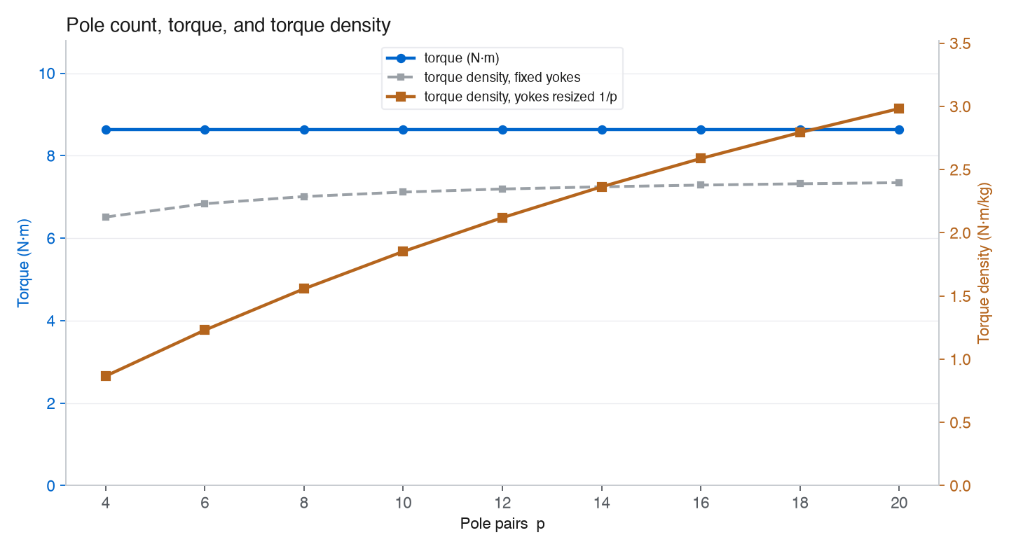
Sweeping pole pairs at a fixed operating point. Torque holds at 8.6 N·m. With the geometry fixed, torque density barely moves; resizing the yokes to each pole count (relative to the p=14 reference) raises it about threefold. From the package’s analytical layer.
The sweep holds the geometry fixed and varies the pole pairs, and torque is flat. The payoff from more poles is torque density: each pole returns less flux, so the yoke can be thinner. Resizing the rotor back iron and stator core with pole count, holding yoke flux density constant, leaves torque unchanged and raises torque density about threefold. Higher pole counts also raise the electrical frequency, which adds core and switching loss at a given speed.
From a point to a trade space
A single evaluation is a starting point. The design question is which compromise to take, and that needs the trade space. The optimization layer runs a Pareto study over outer radius, pole pairs, air gap, and fill factor, with three objectives (torque density, efficiency, mass) and the model’s built-in constraints. Every point it returns is feasible.
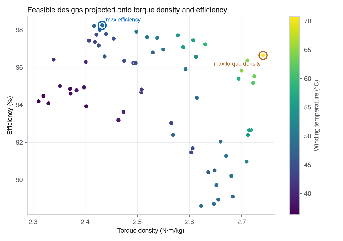
Feasible designs over outer radius, pole pairs, air gap, and fill factor, colored by winding temperature. The highest torque-density designs run hottest; the most efficient design sits at lower torque density. Mass is a third objective, so some points that look dominated here are not dominated once mass is counted. The efficiencies come from the analytical layer, which omits AC, eddy-current, and PWM losses, so they read high.
The torque-density champion and the efficiency champion are different machines, and the torque-density end runs hotter. Picking a design means choosing a place on the front and reading what the constraint margins give up. That logic extends past the motor: the same OpenMDAO wiring lets the actuator be optimized together with its gearbox, inverter, and structure instead of one piece at a time.
The 2.5D layer adds detail the mean-radius model cannot. Because the pole pitch widens with radius, the stator yoke carries more flux toward the outer edge, so the outer radius is where saturation binds first as current loading rises.
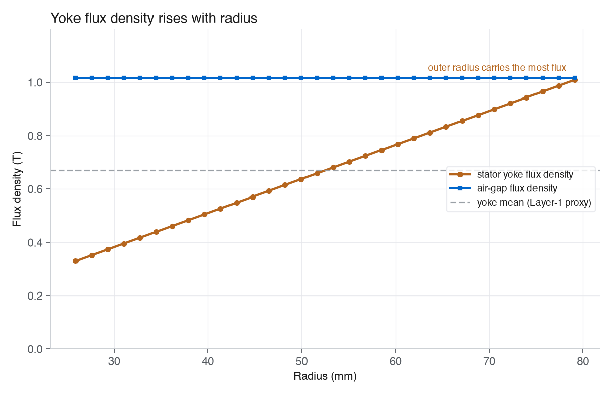
The annular layer resolves fields by radius. The pole pitch widens outward, so the stator yoke flux density climbs from about 0.3 T at the inner radius to 1.0 T at the outer radius while the air-gap field stays flat. The mean value (dashed) is what the analytical layer uses, so it underestimates the most heavily loaded outer radius.
Where the models stop
These models stay fast by leaving physics out, and the package documents what is missing.
- The model is single-gap (one rotor disk, one stator disk). It does not cover the double-gap TORUS, YASA, and AFIR topologies common in high-performance designs. A single-sided rotor also carries a large unbalanced axial pull (about 5 to 6 kN for the reference motor) that the bearing stack has to take; the annular layer reports that axial force.
- There is no magnetic saturation in the torque calculation, so torque is linear in current. The 1D magnetic load line is an upper bound; a finite-element check measured the under-magnet mean air-gap field about 11% lower and the fundamental about 7% lower.
- The voltage constraint neglects the inductive drop, which makes it optimistic when the electrical frequency is high and the bus margin is tight.
- The thermal model is a single lumped resistance to ambient, with no speed-dependent cooling, and the magnet temperature is held at a fixed offset rather than solved.
- AC copper loss, magnet eddy-current loss, and PWM harmonic loss are omitted.
These assumptions are written down and, where it matters, measured against finite element. A fast model is worth keeping when you can see its assumptions, check its residuals, and read its output as an early-stage estimate.
Try it
The package is on PyPI:
pip install "axfluxmdo[opt]"The repo has eight worked examples (analytical evaluation, the pole-pair study, an efficiency map, air-gap sensitivity, torque-density optimization, Gmsh export, Bayesian optimization, and a 3D animation), 24 test files, and a documentation site. The repo and the project page have the rest.
The figures come from the package’s analytical and 2.5D layers on one illustrative motor geometry; they show the method rather than a validated motor. axfluxmdo is early-stage open-source software, and the references are public.
This is an independent project I work on in my own time, using the public sources cited above. The views are my own and do not represent any current or former employer.
More in Modeling & simulation
- sysml2kit 0.4.0: multi-fidelity verification on a compute budget · 2026-08-21
- Track accuracy is an aperture decision · 2026-08-18
- Power-aperture, and the heat it hides · 2026-08-13