Modeling phased arrays in Python, from physics to trade study

2026-06-22

A phased array points a beam by setting the relative phase across many antenna elements, or a true time delay in wideband systems, with no moving parts. As digital arrays have spread, many engineers now work on them without an antenna background, a point Analog Devices makes at the top of its phased-array primer. The beam pattern is the visible part of the design, and the easy part. The harder question is whether a given array meets its system margins: link budget, radar detection range, RF-chain noise, cost, power, and reliability.

I maintain two small open-source tools that split along exactly that line. phased-array-modeling computes the radiation pattern (project writeup here), and phased-array-systems runs requirements-driven trade studies on top of it. This post walks the ladder from one to the other, with an X-band 16×16 array as the running example. Every figure is generated from these two libraries.

From elements to a beam

Put N elements at known positions and give each a complex weight. The far-field array factor is the sum of those weights, each turned by the phase the wave picks up traveling to its element in a given direction. Steer the beam by setting the weight phases to a ramp matched to the direction you want; that ramp is the steering vector. In the usual approximation of identical elements, the total pattern is the element factor times the array factor (Analog Devices, Part 1): the array factor is what beamforming controls, and the element factor is a fixed envelope that rolls off toward the horizon.

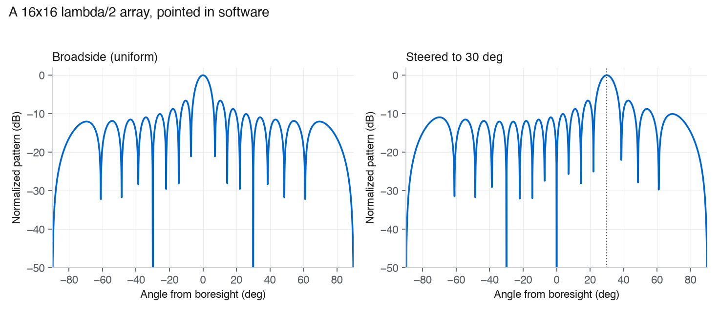
Two principal-plane cuts of a 16 by 16 array: a broadside beam at 0 degrees and the same array steered to 30 degrees — A 16×16 λ/2 array at broadside and steered to 30°. Only the element phases change between the two.

Scanning off broadside is not free even with ideal hardware. As a planar aperture steers away from boresight, its projected area shrinks, so the beam broadens roughly as 1/cos θ and the directivity falls roughly as cos θ, the usual scan loss (MIT Lincoln Laboratory). The cuts in this post show the array factor; a real element pattern would taper the envelope further toward the horizon.

One catch worth naming early: steering with a phase shift rather than a true time delay makes the beam direction drift with frequency, an effect called beam squint (Analog Devices, Part 2). It is small for narrowband waveforms and grows with bandwidth.

Spacing, tapers, and grating lobes

Element spacing is the first design choice that can ruin a pattern. If the spacing grows past about half a wavelength for a wide scan, the array aliases the wavefront in space and a full-strength copy of the main beam appears in the array factor at another visible angle (the element pattern can suppress it somewhat). That copy is a grating lobe, and it is spatial aliasing in the same sense a sampled signal aliases in time (Analog Devices, Part 2; MIT Lincoln Laboratory). For a uniformly spaced linear array, or a principal-plane cut through a planar one, a useful grating-lobe-free condition is d/λ < 1/(1 + |sin θ_scan|). Half-wavelength spacing is the standard rule of thumb because it avoids visible grating lobes across the ideal scan hemisphere; real arrays rarely scan usefully to the horizon, because element pattern, scan loss, coupling, and packaging intervene.

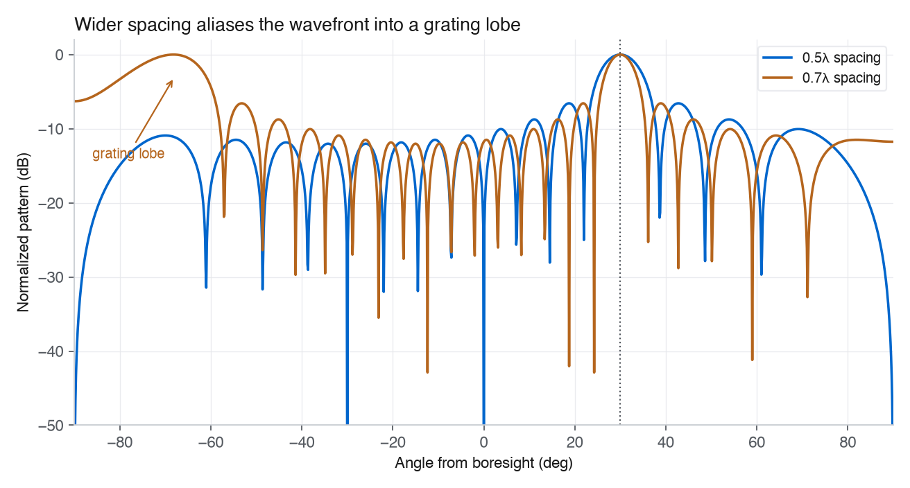
Two pattern cuts steered to 30 degrees: 0.5 wavelength spacing has one main beam, while 0.7 wavelength spacing grows a second full-height grating lobe near minus 68 degrees — Both arrays are steered to 30°. At 0.7λ spacing a grating lobe appears near −68°; at λ/2 it does not.

The second choice is amplitude tapering. Weighting the elements toward the center, for example with a Taylor taper, lowers the sidelobes that sit beside the main beam. The cost is a wider main beam and a small loss in gain, the taper efficiency.

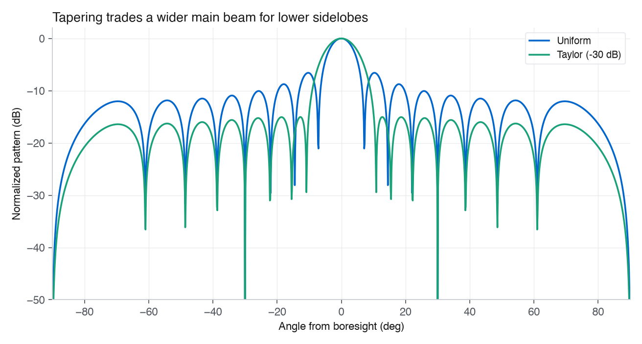
Broadside pattern cuts for uniform versus Taylor minus 30 dB weighting; the Taylor taper has much lower sidelobes and a slightly wider main beam — A Taylor (−30 dB) taper drops the sidelobes well below the uniform case and widens the main beam.

What real hardware does to the pattern

The patterns above assume ideal phase and amplitude at every element. Real arrays do not get that.

Phase shifters have a finite number of bits, so the steering phases snap to a few discrete levels. Coarse quantization raises the sidelobe floor and can throw quantization lobes. By four bits the pattern is close to ideal in this example, and at two bits the sidelobes climb sharply; quantization sidelobes are angle-dependent and improve by about 6 dB per bit (Analog Devices, Part 3).

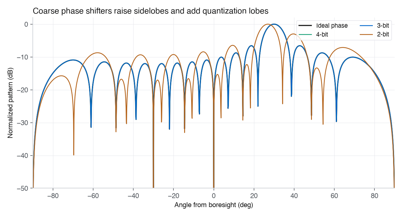
Pattern cuts steered to 30 degrees for ideal phase and 2, 3, and 4 bit phase quantization; the 2-bit case has much higher sidelobes — Phase quantization steered to 30°. Three- and four-bit shifters track the ideal pattern; two bits do not.

Elements also fail. Transmit/receive modules die over a long deployment, and the array has to keep working. The main beam survives a scattering of failures; what rises is the sidelobe floor, which is why large arrays are said to degrade gracefully.

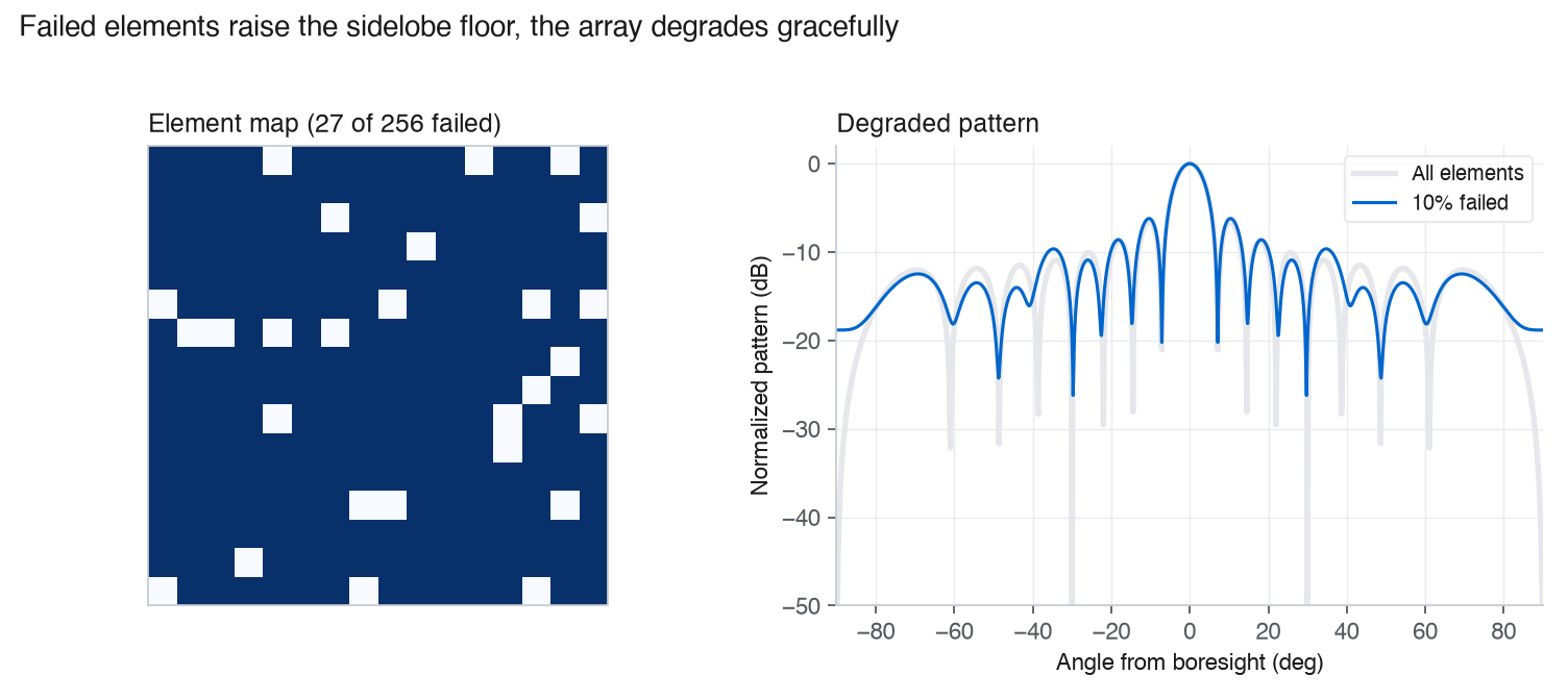
Left: a 16 by 16 element map with about 27 failed elements marked. Right: the pattern with all elements versus 10 percent failed, showing a higher sidelobe floor but an intact main beam — Ten percent of elements failed at random. The main beam holds; the sidelobe floor comes up.

A harder effect to model is mutual coupling. Elements interact in the near field, so each element’s active impedance changes with scan angle. That can cause scan blindness and limits the usable scan volume and bandwidth (MIT Lincoln Laboratory). The library includes coupling and scan-blindness models, but it treats them as engineering approximations. They do not replace full-wave electromagnetics or a measured active-element pattern.

From pattern to system margin

A clean pattern is necessary and far from sufficient. The second library turns array choices into the metrics a system is actually judged on.

For a communications link it computes EIRP and link margin: EIRP combines the per-element power with the array gain, and the margin is the received SNR minus the SNR the link requires. For radar it uses the monostatic radar equation,

SNR = (Pt · G² · λ² · σ) / ((4π)³ · R⁴ · k · T · B · L)

where the range enters as R⁴, because the signal spreads on the way out and again on the way back (MIT Lincoln Laboratory). That fourth power is why doubling detection range needs roughly sixteen times more in the radar-equation numerator: transmit power, antenna gain, integration gain, target RCS, or some combination. For the receiver it cascades noise figure (Friis), third-order intercept, and dynamic range down the RF chain.

The point of all this is that one array decision reads differently at the two levels:

Array choice	What it does to the pattern	What it does to the system
Larger aperture	narrower beam, more gain	better link and radar margin; more cost, power, weight
Amplitude taper	lower sidelobes, wider beam	less interference and clutter; slight gain loss
Wider element spacing	grating-lobe risk	cheaper aperture; smaller usable scan volume
More power per element	pattern unchanged	more EIRP and SNR; more heat and DC power
Tolerating failed elements	higher sidelobe floor	graceful degradation; reliability margin

From a single design to a trade space

A single design is one point. The object worth reasoning about is the trade space around it. The systems library samples a design space with a Latin-hypercube DOE, evaluates each design against the requirements with pass/fail and margins, filters to the feasible set, and extracts the Pareto frontier.

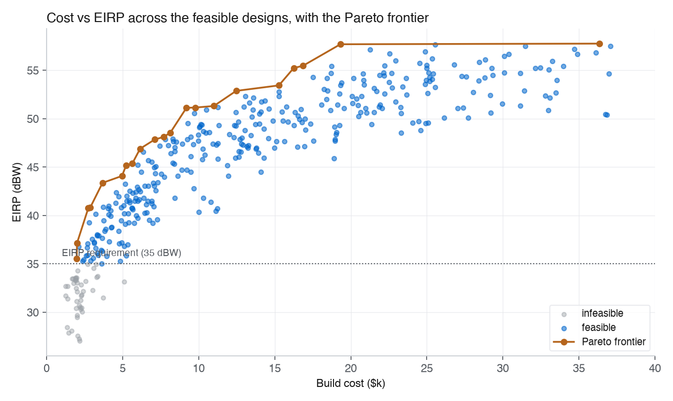
Scatter of build cost versus EIRP for many sampled designs, with infeasible designs below the 35 dBW requirement line, feasible designs above it, and a Pareto frontier tracing the best cost-EIRP tradeoff — Build cost against EIRP for a swept design space. Designs below the EIRP requirement are infeasible; the frontier traces the cheapest design at each EIRP. Cost and EIRP here use simple first-order models.

The frontier has a knee. Past it, more EIRP costs disproportionately more money, and the best-looking pattern is rarely the cheapest design that still clears the requirement. That is the question a pattern plot alone cannot answer.

Where this model breaks

A first-order model earns trust by being clear about its limits.

phased-array-modeling models the array factor and synthesizes patterns. It is not a full-wave solver: not HFSS, CST, or FEKO, and not measured chamber data or a calibration model.
The mutual-coupling and scan-blindness models are illustrative approximations. Real scan performance can be dominated by coupling that needs full-wave simulation or measurement.
The radar detection model (Albersheim, Marcum-Q, Swerling, CFAR) is first-order. Real performance depends on waveform design, processing, calibration, clutter statistics, and validation data.
The cost and EIRP numbers in the trade study use simple models for array gain and unit cost. They show the method. The numbers are not a price for any real system.

A first-order model earns trust by failing in understandable ways, and the limiting cases here all check out: λ/2 spacing avoids visible grating lobes across the ideal scan hemisphere, wider spacing eventually aliases, a taper trades sidelobes for beamwidth and gain, off-boresight scan broadens the beam and lowers directivity, and the radar equation punishes range as R⁴. The value of the model is that those checks are easy to run; high fidelity is a separate job.

Everything here is built from public open-source code and textbook physics. There are no classified or proprietary performance claims.

Try it

Both libraries are on PyPI:

pip install phased-array-modeling phased-array-systems

The pattern library has a browser demo for steering and geometry, and the systems library ships trade-study examples you can run directly. The code, with the array model and the system trade studies, is on GitHub: phased-array-modeling and phased-array-systems. If you think a number or an assumption is off, the math is all visible, and I would like to know.

The figures are generated from the two libraries on an illustrative X-band 16×16 example. The cost and link-budget numbers use simple first-order models and are not a design for any real system. The references are public.

This is an independent analysis I did on my own time, using the public sources cited above. The views are my own and do not represent any current or former employer.