Power-aperture, and the heat it hides
Five agent-generated designs passed the search-radar task in my benchmark. Their per-element transmit power ranged from 4 W to 9 W. Their apertures ranged from 1600 to 2304 elements, arranged 40 × 40, 48 × 48 and 64 × 32. By every knob the task exposed, they are different machines.
When I finally computed how much heat each one dumps per square centimetre of array face, the five collapsed onto two values: 0.472 W/cm² and 0.518 W/cm².
That clustering is a warning. It means the quantity was pinned by something none of the designs was reasoning about, and my model could not have said so, because until last week it never computed an area.
The line that was missing
The whole thermal chain in phased-array-systems came down to one expression:
heat_per_elem_w = max(0.0, dc_power_w - rf_avg_power_w) / n_elements
junction_temp_c = ambient_temp_c + thermal_resistance_c_per_w * heat_per_elem_w
Divide the dissipated power by the element count, push the result through a lumped junction-to-ambient resistance, feed the temperature to an Arrhenius derating model. It is a per-device normalization, and it answers a real question: how hot does one transistor get.
Element spacing appears nowhere in it. Pack the elements twice as close and this model reports
an identical junction temperature, while the physical array now has four times as much heat to
pull through the same cold plate. ArrayConfig stores spacing in wavelengths and carries no
frequency at all, so a physical aperture in square metres was never formed anywhere in the
package. Meanwhile the thermal resistance itself was a free input: 40 °C/W in the search-radar
task, asserted by the task author, with nothing checking that a cooling path of that quality is
achievable at the heat flux the design actually produces.
I went looking across all seven repositories in this ecosystem. Zero hits for watts per square
centimetre, watts per square metre, or heat flux in the areal sense. Three near-misses exist and
are easy to confuse with the real thing: pa_psat_w_per_mm is semiconductor power per unit gate
periphery, a device property; resolution_cell_m2 in the clutter model is a patch of ground; and
the “power density” in my radar-equation documentation is far-field flux at a target, falling as
1/R². None of them is power per unit area of array.
Two numbers bracket a search array
For volume search, the top-level figure of merit is the product of average transmit power and effective aperture area:
Look at what is absent from the right-hand side. Frequency does not appear. Antenna gain does not appear. A higher-frequency array of the same physical size has more gain per beam, and needs proportionally more beams to cover the same search volume, and the two effects cancel exactly. The search requirement is therefore independent of wavelength. The MIT Lincoln Laboratory radar course puts it on the slide that scales this equation: the power required is “Independent of wavelength.” Skolnik’s Radar Handbook adds the qualification worth keeping, that frequency is absent only explicitly and re-enters implicitly through the other terms. It comes back through everything the equation does not show you, including the heat.
This is why power-aperture is the right quantity to argue about first. It compresses range, revisit rate, search volume and target size into one number with units of W·m², and it tells you nothing about how to build the thing. Required power-aperture scales as , and as search volume divided by frame time, so halving the revisit time doubles what the mission demands.
The second number is what stops you from buying that product the cheap way. Dissipated power per unit aperture area:
At half-wave spacing the cell is , so at fixed dissipation per element
I went looking for a published source that states this scaling directly and did not find one, which surprised me. The nearest is a Northrop Grumman patent on Ka-band array design, which observes that element spacing above 30 GHz leaves a cell under a tenth the area of one at 10 GHz. That is the same fact approached from the geometry side.
Those two quantities are dimensional inverses. Power-aperture is watts times area; heat flux is watts per area. One says the mission needs more of the product. The other constrains how tightly that product may be packaged. A design optimized against either one alone comes out oversized or unbuildable.
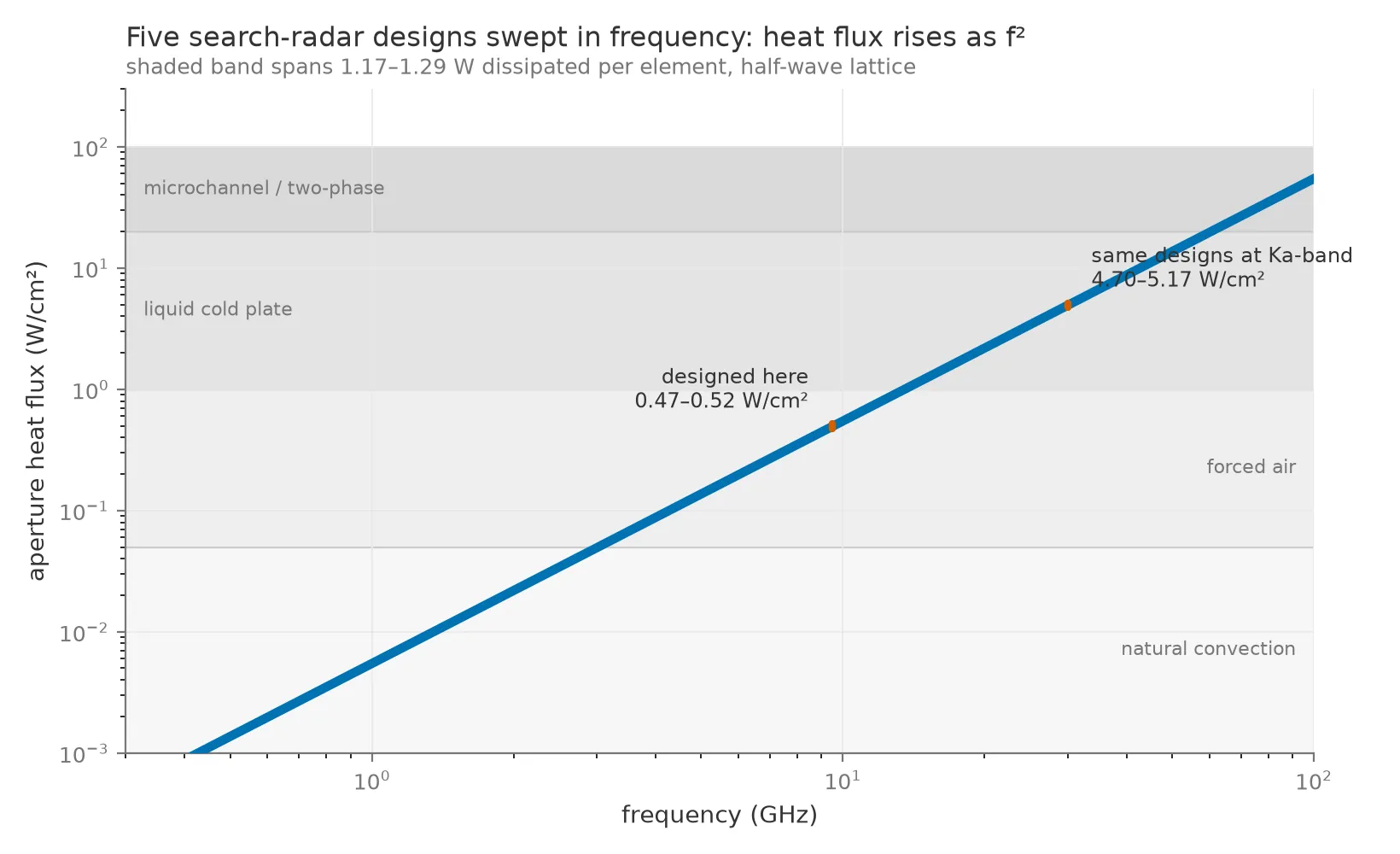
The five recorded designs, swept in frequency at their own half-wave lattice. Only their dissipated power and lattice geometry are data; cell area, aperture area and heat flux are recomputed by the figure script, and the cooling thresholds are read from the library’s cited catalog so the figure cannot disagree with the code. Nothing about the designs changes between the two markers except the band they operate in.
What the numbers said about my own designs
Here are the five, evaluated through the library that now computes all of this. The last column re-evaluates the identical architecture at 30 GHz.
| Array | Elements | P/element | Dissipated | Cell area | q″ at 9.5 GHz (W/cm²) | q″ at 30 GHz (W/cm²) |
|---|---|---|---|---|---|---|
| 64 × 32 | 2048 | 6 W | 2405 W | 2.490 cm² | 0.472 | 4.703 |
| 64 × 32 | 2048 | 8 W | 2404 W | 2.490 cm² | 0.472 | 4.703 |
| 48 × 48 | 2304 | 4 W | 2705 W | 2.490 cm² | 0.472 | 4.703 |
| 48 × 48 | 2304 | 9 W | 2971 W | 2.490 cm² | 0.518 | 5.165 |
| 40 × 40 | 1600 | 7 W | 2063 W | 2.490 cm² | 0.518 | 5.165 |
The ratio between the last two columns is 9.972 for every row. The predicted ratio, (30/9.5)², is 9.972. The algebra predicts it; these are five designs where it holds.
The clustering in the second-to-last column has a mundane explanation, and it is the interesting part. The task carries an availability requirement, which the reliability model enforces through junction temperature, which pins dissipation per device. Every one of the five designs chose 0.5λ spacing, so cell area was a constant 2.490 cm² across the set. Heat flux is dissipation per device divided by cell area, and with both pinned there were only ever going to be a couple of answers.
So in this particular task, junction temperature was acting as a proxy for heat flux. That proxy holds only because the spacing never varied. Give an agent a reason to thin the array to 0.7λ and the two quantities separate immediately, with junction temperature reporting no change at all while heat flux drops by half.
I want to be direct about what this feature did not do. It would not have rejected any of these five designs. All of them sit comfortably inside forced-air capability, and the full benchmark suite passes unchanged against the updated library, which is the guarantee that the published calibration is still valid. The last column is where the metric earns its place.
The ladder is discrete
Cooling capability does not degrade smoothly. It comes in classes, and the gap between them is paid in hardware.
| Class | Gate | Basis |
|---|---|---|
| Natural convection | 0.05 W/cm² | judgment |
| Forced air | 1 W/cm² | quoted |
| Single-phase liquid cold plate | 20 W/cm² | judgment |
| Microchannel, jet or spray, two-phase | 100 W/cm² | judgment |
Going from forced air to a liquid cold plate adds pumps, a heat exchanger, plumbing, coolant mass, leak paths and a maintenance burden. It is a program decision. That discreteness is exactly what makes the quantity useful in a trade study: it converts a smooth continuum of design choices into a small number of buckets, and tells you which bucket you just landed in.
The cost of getting this wrong is large because the heat is large. Across these five designs, between 54% and 62% of the prime power ends up as heat, so the array dissipates 1.2 to 1.7 W for every watt it radiates. All of that has to leave through the aperture structure, which is why the thermal path drives the mechanical design of an active array.
That ratio swings hard on module efficiency, and it is easy to find far worse numbers. Gaitanakis and colleagues, working from a 20% overall T/R module efficiency, estimate four kilowatts of waste heat for every kilowatt transmitted. My designs sit closer to 38% overall, which is the entire difference between their figure and mine. Either number is meaningless quoted without the efficiency it assumes.
Duty cycle is where this becomes a purchasable trade. Average power is what the cold plate sees; peak power is what sets instantaneous field strength. Raising duty cycle raises average power linearly, which raises the heat the cold plate must remove linearly and raises detection range as the fourth root. Going from 10% to 20% duty at fixed peak power buys about 19% more range and costs exactly double the heat. The same authors work this through for two fighter radars they assume share an aperture, estimating 47 nautical miles at 10% duty against 64 at 20%. Their ratio is steeper than the fourth root of average power alone would give, and the reason matters: raising the pulse repetition frequency raises both the average power and the number of pulses in a dwell, and whether that counts once or twice depends on the integration model underneath. I would check that before quoting the two ranges as a clean duty-cycle trade. Two radars on the same aperture in the same band can therefore differ in detection range purely because one of them has the cooling capacity to run hotter.
Provenance, and where I stopped
Every threshold in the cooling catalog carries a field recording whether I read that number in the primary source or inferred it. The forced-air and cold-plate anchors are quoted verbatim from a DARPA CS MANTECH paper on the ICECool program. The other two are marked as judgment, because the standard open review I wanted to cite for them renders its numerals as embedded objects that three separate text extractors dropped, and I was not willing to quote a number I could not re-read. The regime structure from that review is used; its specific values are not.
I would rather ship a catalog that says “this one is an engineering judgment” than one that looks uniformly authoritative and quietly is not.
Three things adjacent to this are deliberately absent. Die-level and junction-level heat flux run two to four orders of magnitude higher than aperture flux and are governed by spreading resistance through the module, which is a package design problem. RF exposure limits are a siting output; a plane-wave power density cannot establish compliance in the reactive near field of a large array, and a one-metre X-band aperture has a far-field distance near 67 m, so the entire practical hazard zone is near field. Multipaction needs hard vacuum by the standard’s own scope and applies to space missions only.
There is also a transient problem this does not model. Aperture heat flux is reported on average power, because cold-plate time constants are seconds while a radar pulse repetition interval is microseconds. The junction does not average that way: GaN junction thermal time constants are comparable to pulse widths, so within a pulse the junction rises above its pulse-averaged value, and the pulse-to-pulse swing is what drives thermo-mechanical fatigue. The package has no thermal transient model and makes no peak-junction claim.
What I recommend
If you are building a system model for an active array, compute the area. It is four lines of arithmetic and it exposes a constraint that per-device thermal models structurally cannot see.
Compute both ends of the trade. Power-aperture alone will happily hand you an array that meets the search requirement at a heat flux nobody can remove. Heat flux alone will talk you into a sparse, oversized aperture that meets no mission.
Make asserted quantities checkable. The most useful change here was noticing that
thermal_resistance_c_per_w had always been an assertion about a cooling solution that nothing
verified. A design claiming 40 °C/W while demanding 15 W/cm² is asserting
forced-air thermal resistance at cold-plate heat flux, and now the model says so.
Sweep frequency early, even if the band is fixed. The f² scaling means a design that is comfortable at S-band and marginal at X-band is impossible at Ka-band, and the sweep costs one line of code. It is the cheapest way to find out whether your architecture has any headroom in the direction the industry is moving.
Do not add a metric you cannot source. I spent longer verifying four cooling thresholds than implementing the entire feature, and two of them still ended up labeled as judgment. That is an honest outcome.
What shipped
Version 0.12.0 of phased-array-systems adds aperture and cell geometry, dissipated heat flux,
radiated power density at peak and average, a cooling-class feasibility check against the cited
catalog, a junction-temperature limit check reading a maximum that had been sitting in the
technology catalog unread, and the power-aperture product with required-versus-achieved margin.
It also deletes a duplicate energy balance: compute_thermal_load had been dead code with zero
callers while the top-level evaluator inlined a slightly divergent copy of the same formula.
All of it is additive. The golden snapshot gained eight keys and no existing value moved.
pip install "phased-array-systems>=0.12"Every number in this post comes from committed run bundles and library output, recomputed while writing. The cooling thresholds are order-of-magnitude regime gates with their provenance recorded in the repository, and two of the four are engineering judgment rather than quoted values.
The phased-array tools and the benchmark are independent projects I build on my own time. The views are my own and do not represent any current or former employer.
Frequently asked questions
What is the power-aperture product and why does frequency drop out of it?
For volume search the required average power times effective aperture is set by the search solid angle, the frame time, the target cross-section, the required signal-to-noise ratio and the fourth power of range. Antenna gain and wavelength cancel between the transmit and receive sides of the radar equation once you account for the number of beams needed to cover the volume. A higher-frequency array with the same physical area has more gain per beam but needs proportionally more beams to cover the same solid angle, and the two effects cancel exactly.
Why does aperture heat flux scale as frequency squared?
At half-wavelength element spacing each element owns a unit cell of area (lambda/2)^2, which is (c/2f)^2. Hold the dissipation per element fixed and the heat per unit area rises as f^2. Moving a design from 9.5 GHz to 30 GHz multiplies its aperture heat flux by about ten with no other change, which is enough to move it from forced air to a liquid cold plate.
Is heat flux per unit area the same as junction temperature?
No. Junction temperature is a per-device question: take the dissipation in one transistor and push it through a junction-to-ambient thermal resistance. Heat flux is a per-area question: can the cooling approach remove this many watts from each square centimetre of array face. Packing elements more tightly leaves junction dissipation unchanged while raising heat flux as one over the spacing squared, so a model that only computes junction temperature is blind to lattice pitch.
What heat flux can each cooling approach actually remove?
As order-of-magnitude regime gates: natural convection well under 0.1 W/cm2, forced air around 1 W/cm2, single-phase liquid cold plates in the tens, and microchannel or two-phase schemes above 100 W/cm2. DARPA's MACE effort targeted a 10 Kelvin rise at 1 W/cm2 for advanced air cooling, and its Active Cooling Module effort addressed fluxes above 25 W/cm2. These are regime boundaries rather than cliffs, and crossing one is a program decision because it adds pumps, plumbing, coolant mass and leak paths.
Did adding these metrics change any of your published results?
No, and I checked before claiming otherwise. The five recorded designs sit between 0.47 and 0.52 W/cm2, comfortably inside forced-air capability, so the new constraint would not have rejected any of them. The full benchmark suite passes unchanged against the updated library. The metrics matter for designs that have not been run yet, particularly at higher frequency.
More in Modeling & simulation
- sysml2kit 0.4.0: multi-fidelity verification on a compute budget · 2026-08-21
- Track accuracy is an aperture decision · 2026-08-18
- pitchphys, a baseball pitch physics simulator · 2026-07-09