Sizing AI training by its bottleneck resource

2026-06-22

The wrong question

The usual question when buying GPUs is “which one has the most TFLOPs?” Vendor spec sheets lead with a peak compute number, so it is the number people compare. Few real workloads are limited by peak compute alone.

A better question is: which resource limits my workload per token, and what is the cheapest way to buy that resource? The bottleneck moves with the work. Large-batch training matmuls are often compute-bound. Autoregressive decoding is usually memory-bandwidth-bound. A wide distributed run can be network-bound. A big model can be capacity-bound before any of those bind.

Workload	Usual first bottleneck	What to price
Large-batch dense pretraining	compute, sometimes network	$/TFLOP-hour, plus fabric
Decode serving	memory bandwidth and KV cache	$/TB/s-hour, plus memory GB
Wide data-parallel training	network	$/Gbps-hour, plus topology

I wrote a small open model to find which one binds, given a model and a piece of hardware. It is Sizing-AI-Training-by-Cost-per-Memory-Bandwidth: two short notebooks, math and Python, MIT licensed. One result worth noting up front: the model’s own default example, a 70-billion-parameter training run, comes out compute-bound. Even a tool built around memory bandwidth finds plenty of compute-bound cases, which is the point. It tells you which case you are in before you spend money.

The roofline in one picture

The idea underneath all of this is the roofline model (Williams, Waterman, and Patterson, 2009). Attainable throughput is bounded by the smaller of two ceilings: peak compute, and memory bandwidth multiplied by arithmetic intensity. Arithmetic intensity is the FLOPs performed per byte moved.

The crossover is the ridge point, at intensity equal to peak FLOPs divided by bandwidth. Below it a workload is memory-bound and faster compute does nothing. Above it the workload is compute-bound and more bandwidth does nothing.

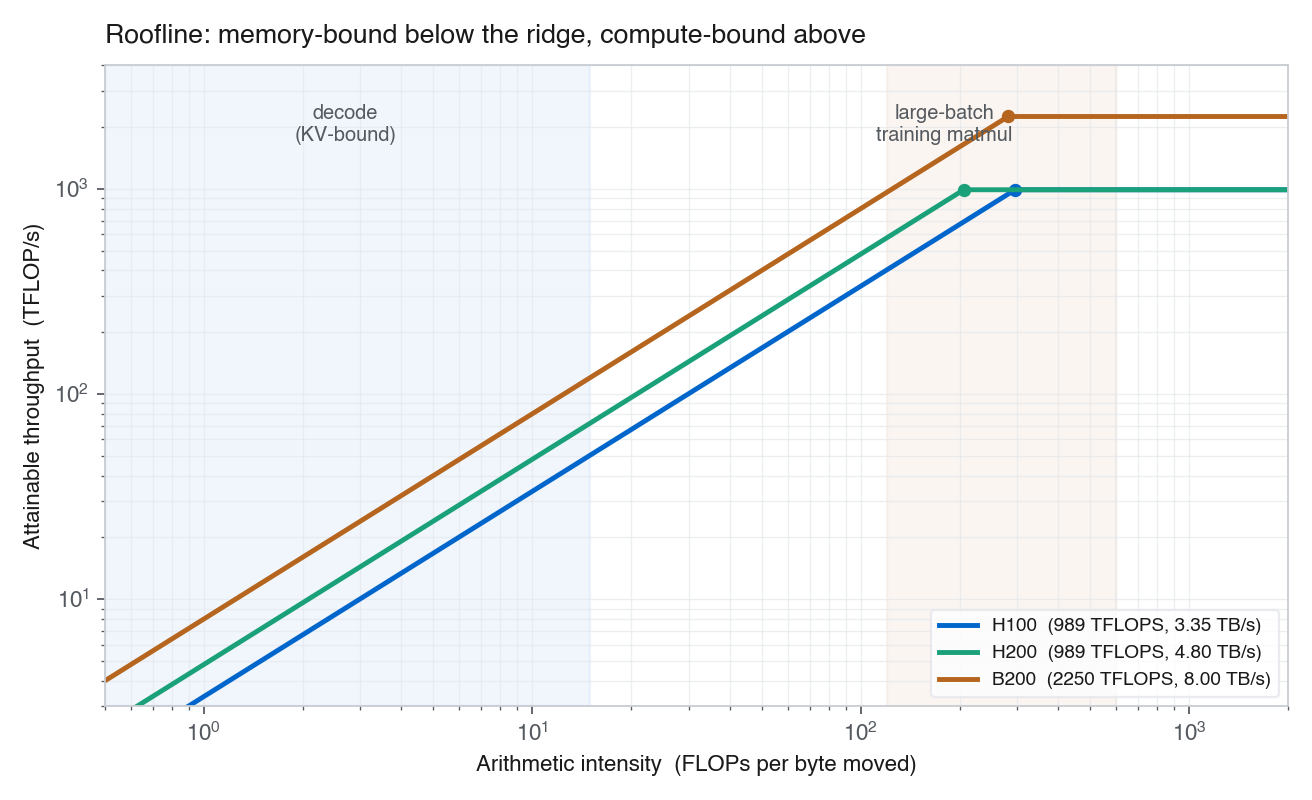
Log-log roofline chart for H100, H200, and B200 showing memory-bound slopes below the ridge and compute ceilings above, with decode at low arithmetic intensity and large-batch training at high intensity — Below the ridge a workload is memory-bandwidth-bound; above it, compute-bound. Decode sits at low arithmetic intensity, large-batch training matmul at high. Peak figures are dense BF16 Tensor Core throughput, with no sparsity doubling.

Where a workload sits on this axis is the whole game. Decode reads a lot of memory per FLOP, so it lands on the left, memory-bound. A well-batched training matmul lands on the right, compute-bound.

Tokens per second as a minimum

The model turns the roofline into a throughput estimate. For a model and a GPU, it estimates the rate each resource can sustain and takes the smallest:

tokens/sec ≈ min( usable FLOPs/sec        / FLOPs per token,
                  usable memory bytes/sec / memory bytes per token,
                  usable network bytes/sec / network bytes per token )

Each term is a supply rate divided by a per-token demand. The smallest term is the bottleneck, and the others have slack. The “usable” fractions matter: vendor peak is never delivered, so the model applies a utilization factor (around 0.75 by default).

For the compute term, dense transformer training costs about 6N FLOPs per token, where N is the parameter count: roughly 2N in the forward pass and 4N in the backward pass (the JAX scaling book derives this). That approximation drops the attention-score FLOPs, which stay small until the context gets long, and it leaves out optimizer math, which is cheap in FLOPs but expensive in memory traffic.

Bytes per token

The memory term is where most of the surprises live, so it is worth accounting for the bytes directly. In training, the traffic per token comes from several places:

parameter and gradient reads and writes
activation traffic, which IO-aware kernels like FlashAttention reduce by keeping work in on-chip SRAM
optimizer state, which dominates memory at scale: mixed-precision Adam carries fp32 master weights on top of two moment buffers, several times the parameter count in bytes, which is why ZeRO exists to shard that state across ranks
gradient communication, an all-reduce across data-parallel ranks; a ring all-reduce moves about 2(p − 1)/p times the gradient bytes per rank each step (NCCL). For a per-GPU rate, divide that by the tokens each rank handles, which is the global batch split across the ranks, so the cost per token grows with the number of ranks
recomputation, where activation checkpointing trades extra FLOPs for less activation memory

Inference is a different regime, and the repo’s second notebook covers it. Prefill is compute-heavy. Decode is memory-bandwidth-bound, because each generated token streams the model weights and reads the KV cache. The KV cache scales as about 2 × layers × KV-heads × head-dim × bytes × context × batch. Grouped-query and multi-query attention cut the KV-head count, which is the main lever for shrinking it.

Cost per bottleneck

Once you know the bottleneck, price the bottleneck. If a workload is memory-bound, the number that matters is dollars per unit of memory bandwidth per hour: price per GPU-hour divided by memory bandwidth in TB/s.

GPU	Memory bandwidth	Representative $/GPU-hour	$/TB/s-hour
H100	3.35 TB/s	~$3.9	~$1.16
H200	4.8 TB/s	~$4.9	~$1.02
B200	8.0 TB/s	~$6.4	~$0.80
L4	0.30 TB/s	~$0.40	~$1.33

The three datacenter parts use HBM; the L4 uses GDDR6, which is why its bandwidth is an order of magnitude lower. B200/GB200-class bandwidth is about 7.7 to 8.0 TB/s depending on the variant.

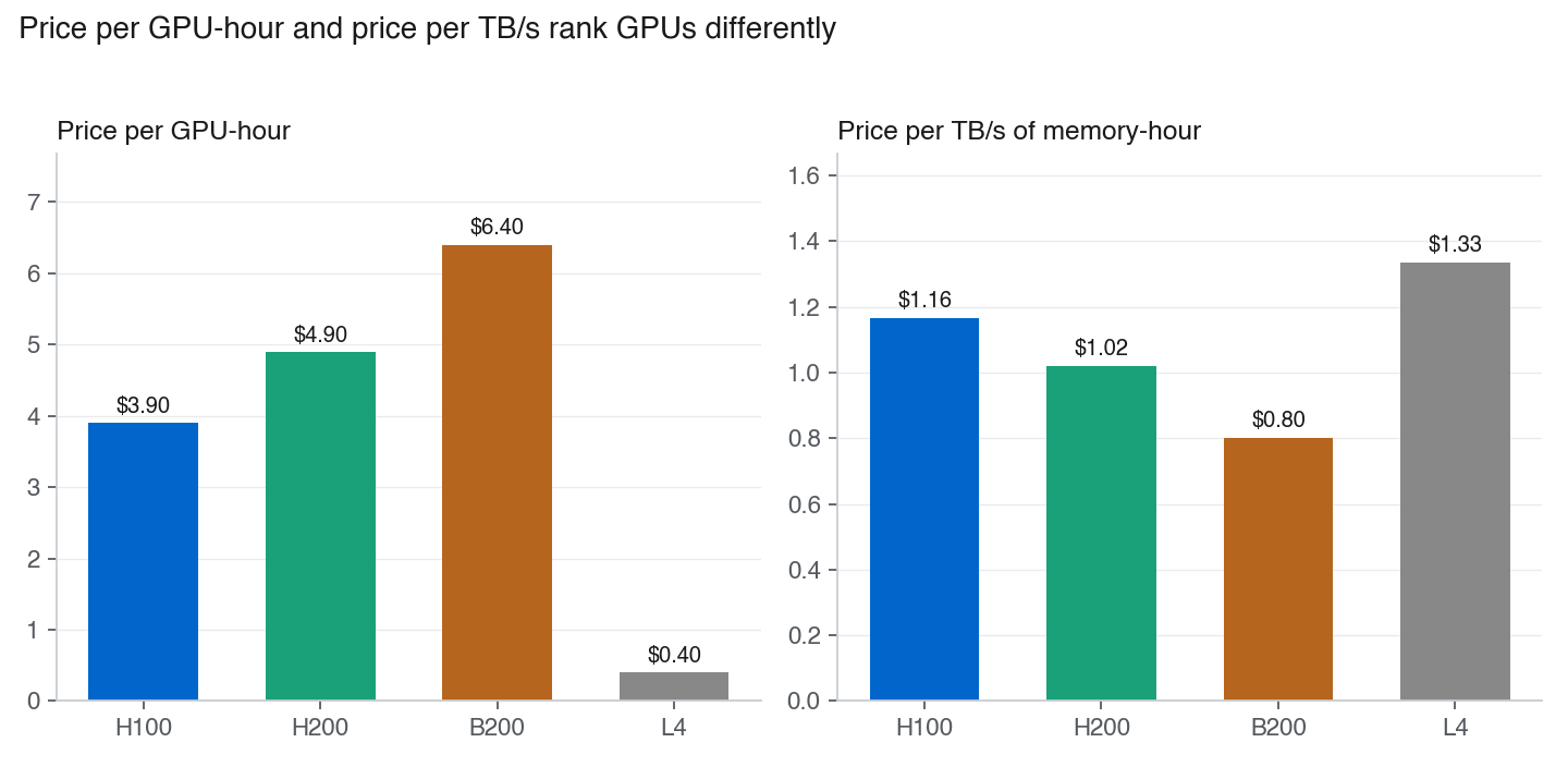
Two bar charts: price per GPU-hour, where L4 is cheapest and B200 most expensive, and price per TB/s of memory-hour, where the order changes so B200 is cheapest and L4 most expensive — The same four GPUs rank differently by absolute price and by price per unit of bandwidth. Prices are representative public on-demand midpoints from mid-2026 across several public GPU clouds and vary widely; the ordering is the signal here, since the exact dollars move week to week.

Two things fall out. The L4 is the cheapest GPU to rent and the most expensive bandwidth to rent, because its memory is small. The H200 and B200 are the bandwidth-cost sweet spots at these prices.

That last point is fragile on purpose. On reserved or committed capacity, the newest flagship is often priced at a steeper premium, which can erase its advantage per TB/s and pull the B200 back level with the H100. So $/TB/s-hour screens candidates; it does not settle the choice. Compute it for the prices you actually face, and read it as one line in a scorecard that also tracks $/TFLOP-hour, memory capacity, network, utilization, and software fit. A B200 that loses on $/TB/s can still win end-to-end on FP4 and FP8 throughput, capacity, and NVLink.

Where this model breaks

A first-order model is useful because it is simple, and dangerous for the same reason. The places it breaks are worth stating plainly:

Vendor peak FLOPs and peak bandwidth are not delivered figures. Real utilization is lower and depends on kernels and access patterns, and it differs by resource: a kernel can reach a high fraction of peak compute while using a low fraction of peak bandwidth, so a single utilization factor is itself a simplification.
Precision comparisons are easy to misuse. FP8 and FP4 throughput numbers are not interchangeable with BF16, and the right one depends on what the workload can tolerate.
Network throughput depends on topology and the collective. Intra-node NVLink and NVSwitch behave differently from inter-node fabric.
Memory capacity can veto a GPU even when $/TB/s looks good. The weights, activations, and KV cache all have to fit.
A larger global batch improves amortization but can degrade optimization, so it is not a free knob.
Mixture-of-experts models need active-parameter and expert-communication accounting, which the total parameter count misses.
Long-context attention breaks the 6N rule, because the attention terms grow with sequence length.

A checklist before you buy

The model is meant to support a decision rather than replace it. A reasonable order of operations:

Name the workload: pretraining, fine-tuning, prefill, decode, MoE, or long context.
Estimate FLOPs per token.
Estimate memory bytes per token.
Estimate network bytes per token.
Compare bottleneck-specific cost: $/TFLOP-hour, $/TB/s-hour, $/GB-memory-hour, $/Gbps-hour.
Validate with one profiled run before trusting the estimate: check delivered tokens/sec, model FLOPs utilization (MFU), achieved memory bandwidth, all-reduce time, and the step-time breakdown.
Then choose hardware.

The notebooks are small and inspectable, with tunable knobs for utilization, optimizer precision, activation traffic, global batch, and the communication check. The repo has the bottleneck-and-cost model and a separate KV-cache sizing deep-dive. If you think a number or an assumption is wrong, the math is all visible, and I would like to know.

Hardware specifications are from vendor datasheets; GPU-hour prices are representative public on-demand figures from mid-2026 that vary widely by provider, region, and commitment. Verify current numbers before making a purchase.

This is an independent analysis I did on my own time, using the public sources cited above. The views are my own and do not represent any current or former employer.