An agentic workflow for phased-array design, from unit cell to link margin
A phased-array design is a chain of assumptions rather than one calculation. The element model feeds the mutual coupling; coupling sets the scan-dependent active impedance; that shapes the array pattern; the pattern sets link margin or radar SNR; and the system margins feed back into how large and how expensive the array has to be. When that chain lives in scattered scripts, a number becomes hard to audit: which assumptions produced it, and at which step?
I built APAB (agentic-phased-array-builder) to make the chain executable and inspectable. It is an LLM that calls a constrained set of phased-array tools and writes down everything it did. I wrote earlier about the array model and the system trade studies these tools wrap; this post is the agent layer on top of them: what APAB is, where it stops, and why the interesting part is the provenance.
The chain of assumptions
The ideal array factor, the sum of steered element weights, is the right place to build intuition and the first thing most tutorials plot. It is also incomplete, and two of the effects it leaves out matter for any real design.
The first is that scanning costs gain even with perfect hardware. As a planar aperture steers off boresight, its projected area shrinks, so the directivity falls roughly as cos θ (Analog Devices, Part 1).
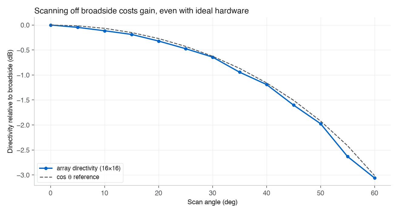
Array directivity falls as the beam scans off broadside, tracking the cos θ scan-loss reference.
The second is that elements are not isolated. Mutual coupling makes each element’s active impedance depend on the scan angle, which is still a live modeling problem for large arrays (arXiv:2601.10982). In the illustrative model here, feeding a coupling matrix back into the excitations perturbs the pattern, filling some nulls and lifting sidelobes.
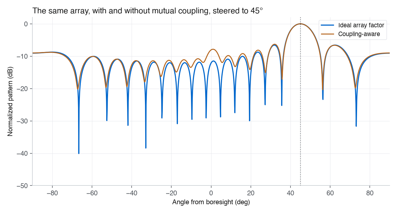
The same array steered to 45°, with and without an illustrative mutual-coupling model.
Neither effect is exotic, and both are why you cannot stop at the ideal array factor. Keeping them straight across a design is bookkeeping, and bookkeeping across a set of typed tools is exactly what an agent is good at.
What the agent actually does
APAB connects an LLM agent to engineering tools through the Model Context Protocol. MCP is an open standard, originally from Anthropic and now stewarded by the Linux Foundation, for exposing tools to language models with typed schemas. Its spec emphasizes validating tool inputs, constraining access, and logging tool use rather than trusting the model, and APAB adds its own workspace-only filesystem and local-first defaults on top. APAB exposes 17 tools that wrap three libraries I maintain: EdgeFEM for full-wave unit-cell simulation, phased-array-modeling for array patterns and impairments, and phased-array-systems for link budgets, radar detection, and DOE/Pareto trade studies. The agent takes a request in plain language, proposes a plan, and calls those tools in sequence: unit cell, then coupling, then pattern, then system metrics, then a report.
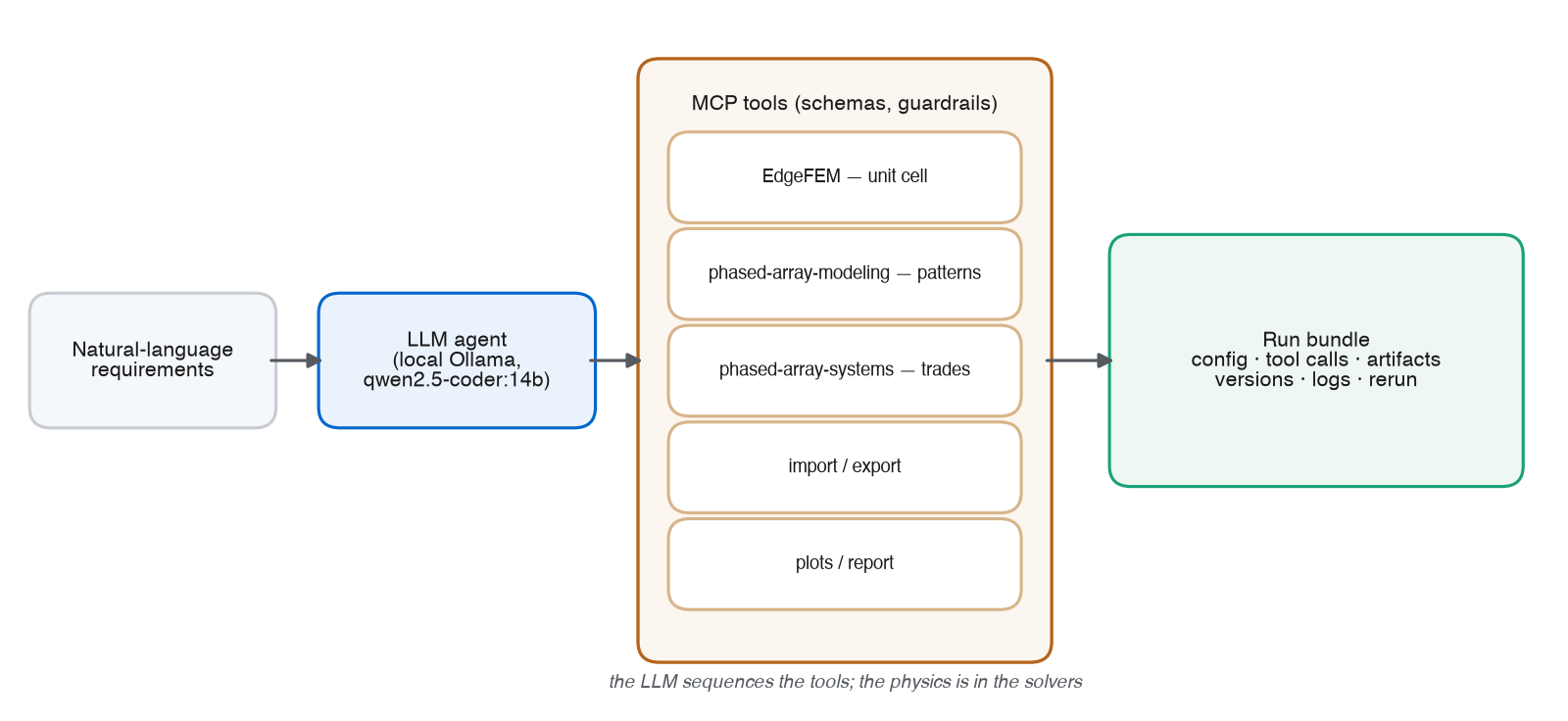
The agent sequences MCP tools; the physics stays in the solvers, and every run produces a bundle.
By default it runs fully local. The provider is Ollama with qwen2.5-coder:14b, so nothing leaves
the machine. Remote providers (OpenAI, Anthropic, Gemini) are opt-in and gated behind a redaction
mode that controls what, if anything, is sent off-box, with audit logs of any egress. The repo ships
a 28 GHz 5G case study that runs the whole chain end to end.
A fair question is why use an agent at all. For a fixed workflow, a script is still the right answer. The agent earns its place when the work is exploratory: sweep a scan range, compare tapers, import a Touchstone file, summarize the active-impedance risk, generate plots, and leave a trace of what happened. The value is making exploratory studies easier to inspect, with a record of every step behind each number.
Where APAB stops
This is the part I want to be plain about, because the failure mode for “AI plus antennas” is overclaiming.
- APAB does not replace HFSS, CST, FEKO, Keysight, or TICRA. Those are mature, validated full-wave and system tools, and a serious design uses them. APAB is exploring what an open, Python-first, local-first agentic workflow around such tools could look like.
- It is not fabrication-ready CAD, and it is not a hosted product. It is alpha-stage v0.x.
- It is not evidence that a language model understands Maxwell’s equations. The LLM sequences tools, chooses which study to run, and proposes inputs; the computed physical quantities come from the solvers and array/system models, or from assumptions stated in the config, rather than from the model’s weights.
- The figures above use illustrative array and coupling models to show why the chain matters; they are not a validated antenna design.
The LLM is the workflow driver. The physics is in the solvers. That division is the whole design.
| Claim | Status |
|---|---|
| 17 MCP tools wrapping EdgeFEM, phased-array-modeling, phased-array-systems | implemented |
Local Ollama (qwen2.5-coder:14b) by default, remote providers opt-in | implemented |
| Unit cell → coupling → pattern → system pipeline | demonstrated (28 GHz case study) |
| Finite-array full-wave validation | future work |
| Figures are validated antenna designs | no, illustrative |
| Replaces commercial EM tools or fabrication CAD | no |
The subtle way a system like this goes wrong is not a badly written sentence. It is silently mixing assumptions: dB against linear power, dBi against dBd, scan-angle conventions, the ideal array factor against an embedded-element pattern, illustrative coupling against measured or full-wave coupling. Typed tools and a recorded run bundle are how I try to keep those mismatches visible.
Provenance is the point
If an agent only hands you an answer, you cannot trust it, because you cannot see how it got there. Recent work on LLM agents argues the same thing: execution traces and evidence, beyond the final answer, are what make an agent’s result accountable (arXiv:2606.04990).
So the useful output of APAB is a run bundle: a directory that records the config, every tool call, the solver inputs and outputs, the plots, the report, the versions, and enough to rerun the whole thing.
workspace/runs/<run_id>/
  manifest.json        # what ran, when, with which tools
  apab.yaml            # the full configuration
  logs.txt
  artifacts/
    coupling/  patterns/  system/  emtool/  plots/  report/
The run manifest records the config, geometry, and sweep hashes, plus the solver and dependency versions and the provider and model names, so a result is tied to the exact code, configuration, and model that produced it. A run that ends in a system trade, for instance, is not a lone plot. It is a Pareto front with its inputs, requirements, and versions attached.
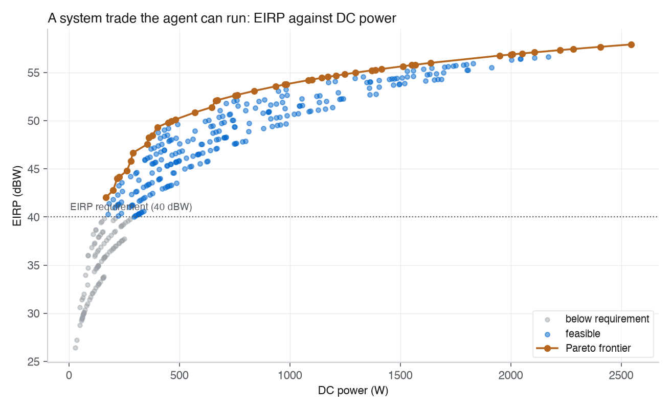
One artifact a run can produce: EIRP against DC power, with the feasible set and a Pareto frontier.
That is the difference between “an AI made a phased array” and a design where every step is recorded, rerunnable, and open to challenge.
Try it
APAB is on PyPI, beta and MIT-licensed. The default provider is local:
pip install "apab[ollama]"
ollama pull qwen2.5-coder:14b   # default local provider
A run scaffolds a project, executes from a config, and writes a bundle you can report on:
apab init --name mmwave_28ghz --dir ./mmwave_28ghz
apab run --config apab.yaml          # batch run; writes a run bundle
apab report <run_id> --config apab.yaml
The repo has the agent, the 17 MCP tool definitions, and the 28 GHz case study; the project page has the short version, and the companion post covers the array and system models the tools wrap. If you think the chain made a wrong turn, the run bundle shows where.
The 0.3.0 release post covers the observability and provenance layer added since this was written: traces of every tool call, run manifests, and a golden-task eval harness.
The figures use illustrative array and coupling models from the underlying libraries; they are not a validated antenna design. APAB is beta-stage software, and the references are public.
This is an independent analysis I did on my own time, using the public sources cited above. The views are my own and do not represent any current or former employer.
More in AI agents
- MCP transport is a lifecycle decision · 2026-08-27
- A SysML v2 model that runs its own verification · 2026-08-21
- Data provenance for agentic AI workflows · 2026-08-17