phased-array-systems 0.9.0: validated physics and multi-objective trade studies
Version 0.9.0 of phased-array-systems is on PyPI, capping a run of three releases that changed what the package is. v0.7.0 made the digital beamforming models accurate (digitization levels, ADC jitter, exact Swerling statistics). v0.8.0 replaced every hand-fit physics approximation with the published model it was imitating, and added a validation suite that proves it. v0.9.0 adds the optimization layer: true multi-objective search, global sensitivity, and constraint-aware design of experiments.
The package is the trade-study layer of the toolchain I wrote about in
modeling phased arrays in Python: it consumes
phased-array-modeling for antenna patterns and answers
system questions (detection range, link margin, cost, power, reliability) against explicit
requirements. It installs as pip install "phased-array-systems[mdao]", imports as
phased_array_systems, and ships a pasys CLI. Docs are at
jman4162.github.io/phased-array-systems.
Physics you can check
The v0.8.0 release notes read like a confession, which is the point. Atmospheric and rain
losses previously came from two-line and polynomial fits; they now come from ITU-R P.676-13
Annex 1 line-by-line gaseous attenuation (79 vendored oxygen and water-vapor spectroscopic
lines) and ITU-R P.838-3 rain coefficients for both polarizations, with no new dependencies.
Sea clutter follows the NRL model fitted to the Nathanson tables, ground clutter the
constant-gamma model. Required radar SNR comes from the exact Marcum-Q inversion instead of
Albersheim’s approximation, which moved the golden regression case from 13.115 to 13.183 dB.
One noise convention now applies everywhere: rx_noise_temp_k is antenna temperature and
T_sys = T_ant + 290(F-1), identical at 290 K and correct for low-sky-temperature satcom cases,
and the radar equation honors the cascaded noise figure the same way the comms path does.
Each of these models is asserted against its published source in a 35-test validation suite, with the references and tolerances documented in the theory section of the docs. The documented approximations that remain are listed as approximations: slant paths use equivalent-height columns rather than layered integration, effective rain path length applies the ITU-R P.530 factor directly, and the CFAR variants beyond cell-averaging use published deltas on the universal curve. A model you can check beats a model that flatters the design.
Optimization joins the loop
Through v0.8, trade studies worked by sampling: generate a design of experiments, evaluate
every case, filter to feasible, extract the Pareto front. v0.9.0 adds the direct route.
optimize_pareto() (in phased_array_systems.trades.moo) runs mixed-variable NSGA-II via
pymoo and returns the nondominated set with full metrics. The constraint handling is the part I
care about: must-severity requirements become normalized inequality constraints, so the
requirement set you already wrote is the constraint set the optimizer respects.
pasys optimize config.yaml --method nsga2 \
  --objective detection_range_m --objective2 cost_total_usd:minimize
pasys sensitivity config.yaml --sens-method sobol --samples 256
Sobol global sensitivity (first-order and total indices, with confidence intervals) answers
which variables move the answer before you spend optimizer iterations on them, and the DOE
generator can now rejection-sample against architecture construction, so batch studies no
longer waste cases on configurations that fail to build. All of it lives behind an [mdao]
extra (pymoo, SALib); the core install is unchanged.
Case study: detection range against cost
The repository’s radar example is a complete requirements-driven study, and everything below
comes from running it as shipped (examples/03_radar_detection_trade.py). The scenario: an
X-band radar at 10 GHz, a 10 dBsm target at 20 km, Pd = 0.9 at Pfa = 1e-6, 16-pulse
noncoherent integration, four requirements defined. The baseline 16x16 array (2560 W peak,
29.1 dB gain) integrates to 16.0 dB SNR against 13.2 dB required, a 2.9 dB margin and 23.6 km
of range at $178,000, and still fails the requirement set.
So the study sweeps: a 15-variable design space (array sizes from 8x8 to 32x32, per-element transmit power from 5 to 20 W, PA efficiency, cost per element), sampled with a 100-case Latin hypercube and evaluated in 0.6 seconds. 49 of 100 designs are feasible, and 8 are Pareto-optimal:
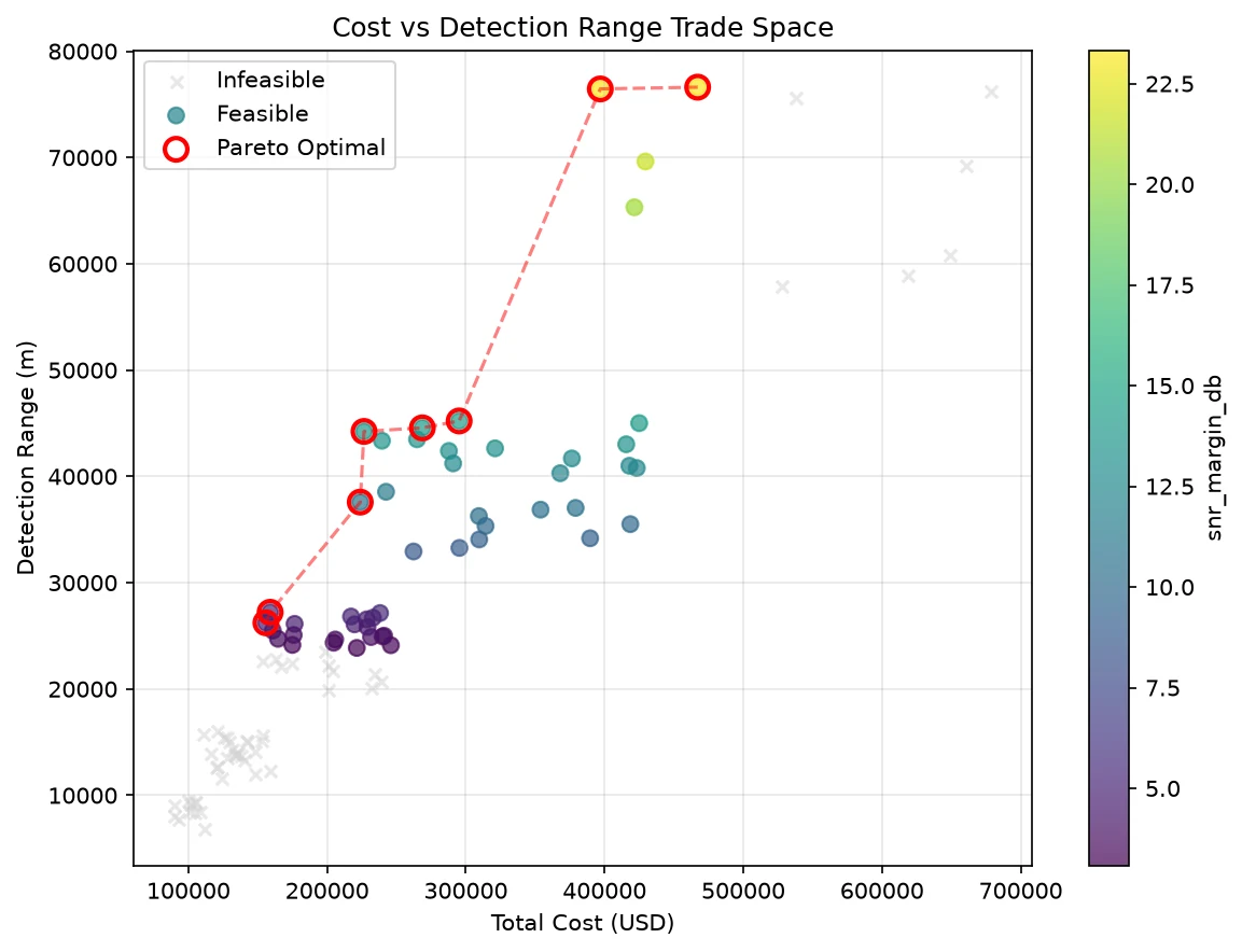
The trade space from the shipped radar example: 100 Latin-hypercube designs, feasibility filtered by the requirement set, Pareto front circled. The front runs from a 16x16 array at 27.2 km and $158,931 to a 32x32 at 76.5 km and $396,945.
The front is the deliverable. At the cheap end, a 16x16 array meets the requirements at 27.2 km and $158,931; the knee sits around 16x32 designs in the mid-40s of kilometers for roughly $225,000; and the 32x32 corner buys 76.5 km and 23.3 dB of margin for $396,945. Every point carries its full metrics dict, so the argument between the $159k and $397k answers happens over named requirements and margins instead of taste.
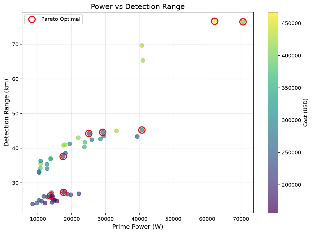
The same study’s power view: detection range against prime power for the feasible designs. A second Pareto front hides in here, which is what the multi-objective path is for.
With v0.9.0, the same study runs through NSGA-II instead of sample-and-filter. The two paths are complementary: the DOE view maps the landscape and feeds Sobol sensitivity, and the optimizer pushes the front itself once you know which variables matter.
Digital beamforming trades
The v0.7.0 layer deserves a mention because it changed what the cost and power numbers mean.
digitization_level (element, subarray, or analog) drives the ADC count, beamformer data rate,
compute load, and DC power from the digitized channel count instead of assuming one ADC per
element. An aperture-jitter model combines with quantization noise into effective ADC SNR, the
system dynamic-range metric includes the array processing gain, and v0.9.0’s
thermal-reliability coupling estimates junction temperature from dissipated power and feeds the
Arrhenius MTBF derating. A dedicated example and tutorial notebook run the
element-versus-subarray-versus-analog architecture trade end to end.
Upgrade notes
- v0.8.0 shifts numeric results by design: real ITU-R losses, Marcum-Q required SNR, one noise convention, and cascaded noise figure in the radar equation.
- Removed:
compute_cost_per_dband the empirical Swerling/CFAR adjustment tables (superseded by exact statistics and the universal curve). friis_noise_figurenow reports per-stage contribution percentages that sum to 100; thecascade_analysiskey is renamedstage_nf_contribution_pct.- Python 3.10+ required; the test suite is at roughly 487 tests with mypy at zero errors as a blocking CI step.
Try it
pip install "phased-array-systems[mdao]"The docs site has the user guide, CLI reference, tutorials, and the theory pages including the validation tables. A Streamlit app wraps the single-case, trade-study, RF-cascade, and radar calculators for browser use:
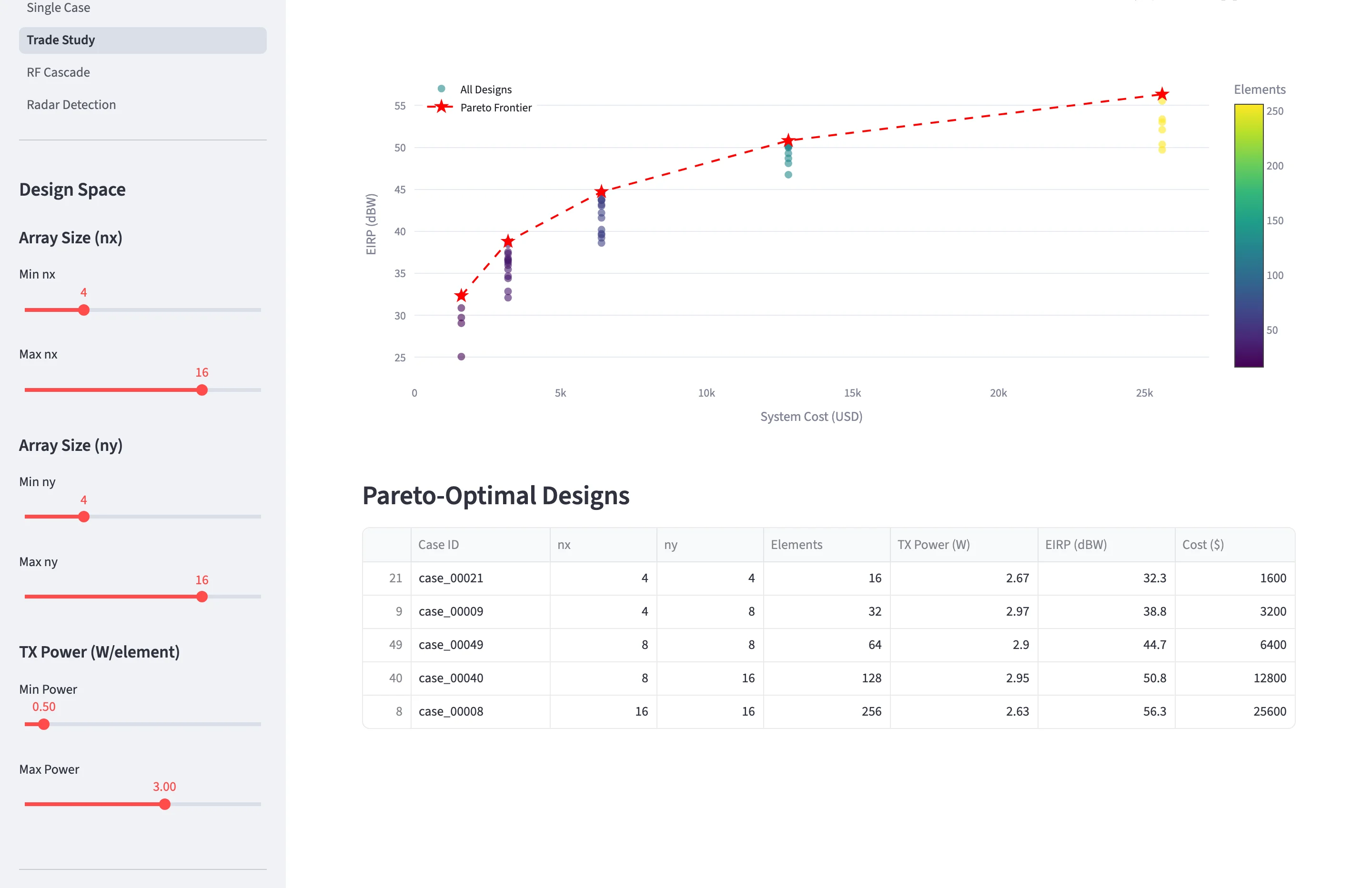
The Trade Study page of the Streamlit app after a 50-design run: an interactive cost-EIRP Pareto frontier and the Pareto-optimal design table.
The repository has the examples used above and Colab-ready tutorial notebooks for the trade-study, DBF-architecture, and MDAO workflows.
phased-array-systems is an independent project I build on my own time. The views are my own and do not represent any current or former employer.
Frequently asked questions
What is phased-array-systems?
An open-source Python package (MIT, CLI pasys) for requirements-driven phased-array system trade studies: comms link budgets, radar detection and search timelines, RF cascade analysis, digital beamforming architecture, thermal-coupled reliability, and cost, swept as designs of experiments and reduced to Pareto fronts. It builds on the phased-array-modeling package for antenna patterns.
What changed in v0.8.0 and v0.9.0?
v0.8.0 replaced hand-fit approximations with published models: ITU-R P.676-13 gaseous attenuation, ITU-R P.838-3 rain, NRL sea clutter, and exact Marcum-Q detection statistics, each verified against its source in a validation suite. v0.9.0 added true multi-objective optimization (NSGA-II via pymoo), Sobol global sensitivity, constraint-aware DOE, and thermal-reliability coupling.
Is the physics validated?
Each model is tested against its published source with documented tolerances (ITU-R recommendations, the NRL clutter tables, CFAR universal curves, Swerling statistics), and the references live in the theory documentation. Documented approximations remain, such as equivalent-height slant columns instead of layered atmospheric integration, and are listed as approximations rather than hidden.
Will my results change when I upgrade?
Likely yes. v0.8.0 shifts numeric results by design: real ITU-R losses replace hand fits, required radar SNR uses the exact Marcum-Q inversion instead of Albersheim, one noise convention applies everywhere, and the radar equation now honors the cascaded noise figure. The golden regression case moved by fractions of a dB; low-sky-temperature satcom cases move more.