OpenEM Wave Lab: an interactive browser lab for electromagnetic wave physics
I released OpenEM Wave Lab, an open-source, browser-based lab for learning how electromagnetic waves behave. It runs live in the browser with nothing to install: drag a slider and the field vectors, phase fronts, power flow, and governing equations all update together, computed from the same model.
The gap it aims at is the one between a textbook and a solver. Textbook figures are static, and most wave animations online are decorative, drawn to look right rather than computed from fields. Full computational electromagnetics tools are built for design work, and they bury the concepts a learner needs under meshing and solver setup. OpenEM Wave Lab, in its own README’s words, “sits between static textbook figures and professional computational electromagnetics software”: every lesson is an analytic or reduced-order model whose parameters you can change and interrogate in real time.
Five modules
Plane wave. A 3D scene of E, H, and k for a uniform plane wave, with a polarization ellipse (linear, circular, elliptical, with IEEE handedness, axial ratio, and tilt) and lossy media that attenuate the fields as they propagate. A movable probe reports phasors, instantaneous fields, Poynting flux, and energy densities at a point. This module is labeled exact: the model is the full closed-form solution, and the visualization adds nothing to it.
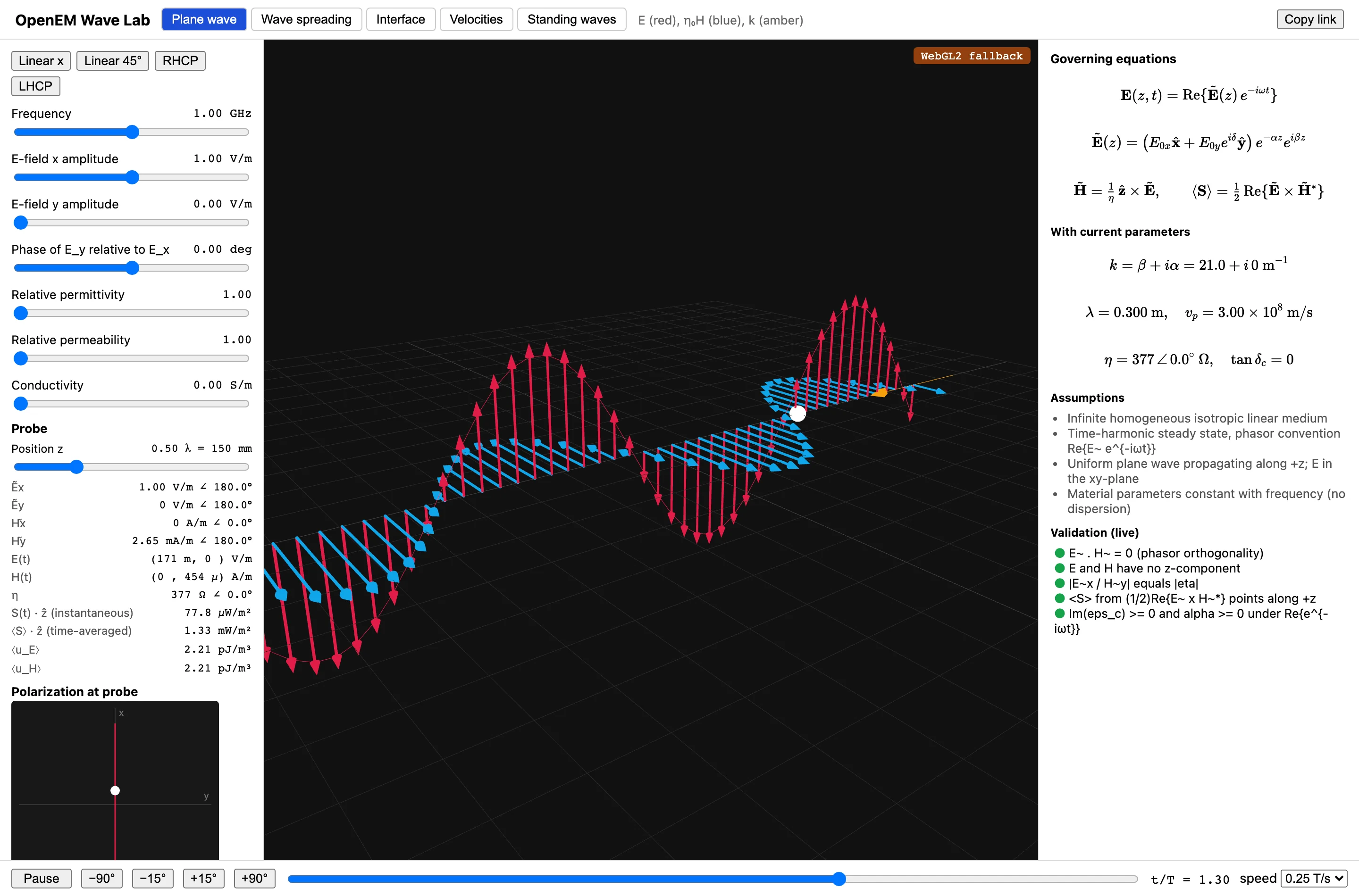
The plane-wave module. The equation panel on the right is computed from the same model as the 3D fields, and the validation checks (phasor orthogonality, impedance ratio, Poynting direction) run live against the current parameters.
Wave spreading. Plane, cylindrical, and spherical waves side by side, with amplitude-versus-radius plots showing the constant, one-over-square-root-of-distance, and one-over-distance falloffs, and a flux check computed from the fields rather than asserted. The cylindrical case uses the outgoing Hankel function, so near-field behavior is right too.
Planar interface. TE and TM Fresnel coefficients at a boundary between two media, with presets for the Brewster angle, total internal reflection, lossy media, and a perfect electric conductor (the PEC case uses the exact mirror coefficients, so there is no large-conductivity approximation). The heatmap shows the continuous field component, which makes the tangential boundary condition visible as smoothness across the interface line, and the evanescent field under total internal reflection is right there to probe.
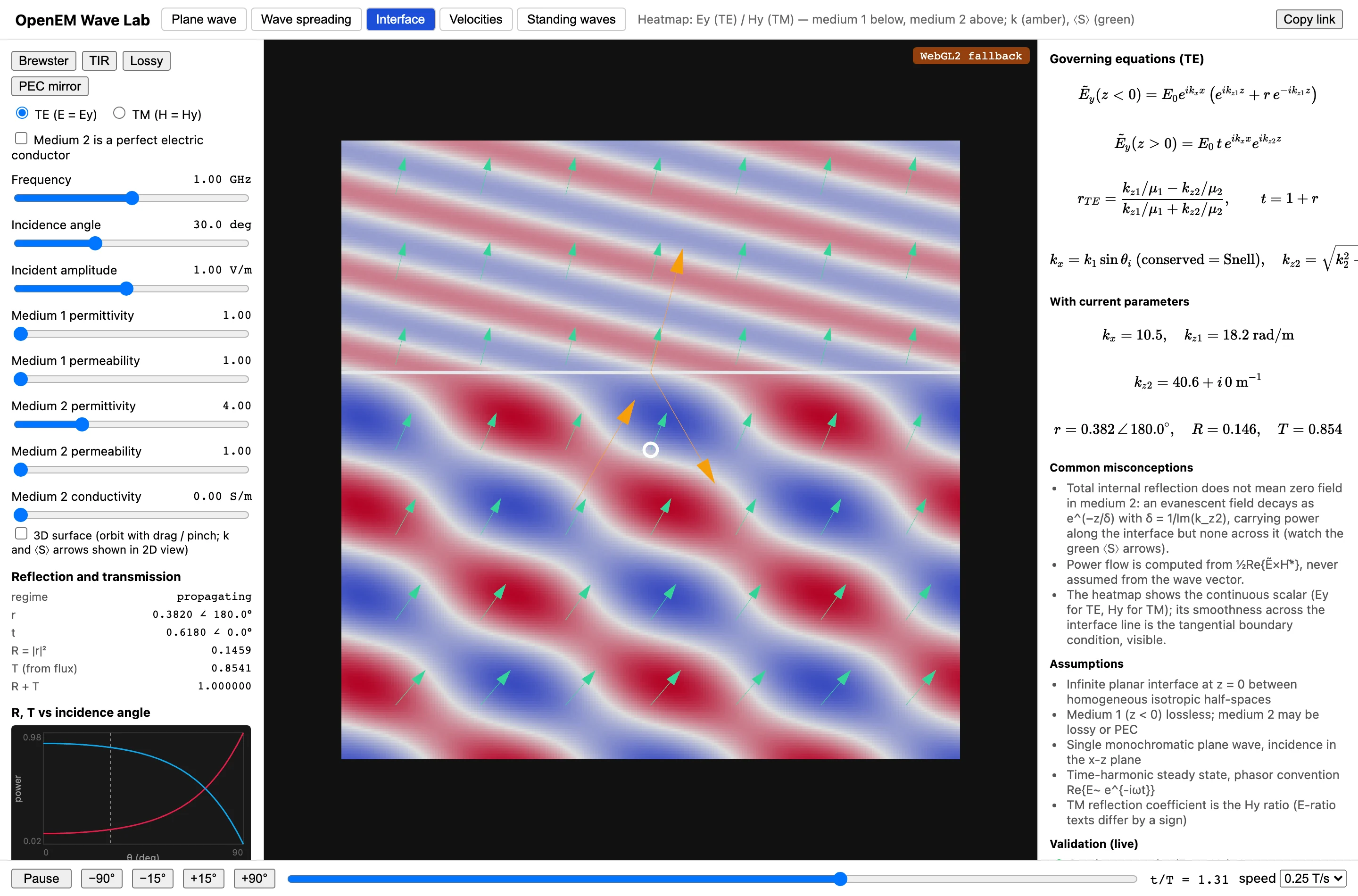
The planar-interface module at 30 degrees incidence into a denser medium. The standing-wave interference above the boundary, the refracted wave below it, and R + T = 1.000000 in the left panel are all computed from the same Fresnel model.
Velocities. Phase, group, and energy velocity in a dispersive medium with waveguide-type dispersion. A crest marker races an envelope-peak marker so you can watch carriers slide through a beat envelope, a Gaussian pulse spreads under group-velocity dispersion, and the dispersion diagram shows phase velocity as the chord and group velocity as the tangent of the same curve.
Standing waves. A forward wave meets a complex reflection coefficient, with short, open, and matched presets, live SWR, and the node structure. A probe makes the classic subtlety concrete: an instantaneous zero crossing of the total field is not a node.
The renderer never touches the physics
The design rule behind the project is separation. All field math lives in a standalone TypeScript package with no dependency on the renderer or the UI, and every module implements one contract:
interface PhysicsModel<State, Sample> {
  id: string;
  fidelity: 'exact' | 'analytic' | 'reduced-order' | 'numerical' | 'conceptual';
  assumptions: string[];
  derive(state): DerivedQuantities;
  sampleField(state, points, time): Sample;
  observables(state, point?, time?): Observable[];
  validate(state): ValidationResult[];
}
Every module declares its fidelity level and its assumptions, and the assumptions render in the
UI next to the scene. Poynting vectors are computed from E cross H, so power flow is a result
you can check rather than an arrow someone drew. The physics package carries 106 test cases
against closed-form identities, limiting cases, conservation laws, and Bessel-function values
from Abramowitz and Stegun, and each model’s validate() runs at runtime so the UI shows a
live checklist (phasor orthogonality, impedance ratios, flux conservation) for the exact
parameters on screen.
One convention holds everywhere: fields are , which puts the conductivity term in the complex permittivity with a plus sign, . Readers trained on the engineering convention of Balanis or Pozar will find those formulas conjugated here, and the lab states the convention in every lesson and pins it with tests. It matters for more than signs: under , the combination is right-hand circular polarization toward +z by the IEEE definition, which is the reverse of what the engineering-convention texts write for the same symbols. Anyone who has debugged an antenna polarization mismatch will recognize why the lab treats this as test-enforced rather than a footnote.
For RF engineering
The modules map onto working RF intuition. The standing-wave module is impedance matching seen from the field side: the complex reflection coefficient, SWR, and node positions that a network analyzer summarizes as return loss. The interface module is the physics under radomes, multipath, and dielectric loading, with the Brewster and total-internal-reflection regimes a slider away. The velocities module is waveguide dispersion, the reason a pulse’s envelope and its carriers travel at different speeds and why group delay varies near cutoff. And the plane-wave module’s handedness and axial-ratio readouts are the same quantities on an antenna polarization spec.
For the computational side of the same subject, my earlier post on modeling phased arrays in Python covers array factors, element patterns, and coupling. This project is the intuition layer underneath that work: what the fields themselves are doing.
Under the hood
The app is a TypeScript monorepo: React 19 for the UI, three.js rendering through the WebGPU
renderer with automatic WebGL2 fallback, zustand for state, and KaTeX for the equation panels.
Every experiment serializes its non-default parameters into the URL, so a specific
configuration (a Brewster-angle setup, a circularly polarized lossy-medium wave) is a link you
can share or bookmark. To run it locally: Node 24+, pnpm 10, pnpm install, pnpm dev.
Status and roadmap
This is an early release: five modules, with negative refraction in causal dispersive materials, whispering-gallery modes, and eventually an FDTD laboratory planned. The code is Apache-2.0 and the written lesson content is CC BY 4.0. Contributions are welcome, with one standing rule from the contributor guide: physics correctness ranks above visual polish, and a change that only looks right in the browser does not merge. Bug reports about the physics get their own issue template asking for the module, the experiment URL, and the displayed versus correct result with a reference.
Try it at jman4162.github.io/openem-wave-lab; the code is at github.com/jman4162/openem-wave-lab.
OpenEM Wave Lab is an independent project I build on my own time. The views are my own and do not represent any current or former employer.
Frequently asked questions
What is OpenEM Wave Lab?
An open-source, browser-based learning tool for electromagnetic wave physics and RF engineering. Five interactive modules (plane waves, wave spreading, planar interfaces, wave velocities, standing waves) compute fields live from closed-form models, with the governing equations, field vectors, and power flow updating together as you change parameters.
Do I need to install anything to use it?
No. It runs entirely in the browser at jman4162.github.io/openem-wave-lab, rendering with WebGPU where available and falling back to WebGL2. Nothing is sent to a server; every experiment state serializes into a shareable URL.
How is the physics validated?
The physics lives in a standalone TypeScript package with no rendering dependencies, covered by 106 test cases against closed-form identities, limiting cases, conservation laws, and published Bessel-function tables. Each module also declares its fidelity level and assumptions, and exposes runtime validation checks that the UI displays live.
Is OpenEM Wave Lab free and open source?
Yes. The code is Apache-2.0 and the written lesson content is CC BY 4.0, on GitHub at jman4162/openem-wave-lab. It is in early development, with five modules shipped and more physics planned.